Time series Decomposition Farideh DehkordiVakil Introduction n n

Time series Decomposition Farideh Dehkordi-Vakil

Introduction n n One approach to the analysis of time series data is based on smoothing past data in order to separate the underlying pattern in the data series from randomness. The underlying pattern then can be projected into the future and used as the forecast.

Introduction n The underlying pattern can also be broken down into sub patterns to identify the component factors that influence each of the values in a series. This procedure is called decomposition. Decomposition methods usually try to identify two separate components of the basic underlying pattern that tend to characterize economics and business series. n n Trend Cycle Seasonal Factors

Introduction n The Trend Cycle represents long term changes in the level of series. The Seasonal factor is the periodic fluctuations of constant length that is usually caused by known factors such as rainfall, month of the year, temperature, timing of the Holidays, etc. The decomposition model assumes that the data has the following form: Data = Pattern + Error = f (trend cycle, Seasonality , error)

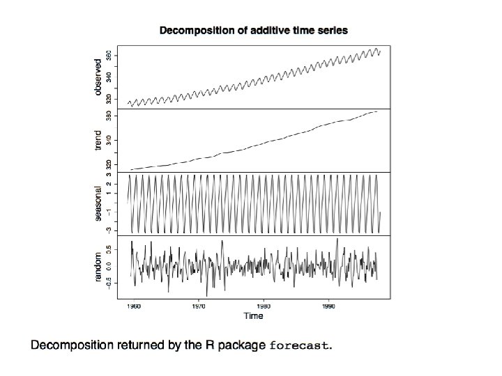
Decomposition Model n Mathematical representation of the decomposition approach is: n n Yt St Tt Et is the time series value (actual data) at period t. is the seasonal component ( index) at period t. is the trend cycle component at period t. is the irregular (remainder) component at period t.

Decomposition Model n The exact functional form depends on the decomposition model actually used. Two common approaches are: Additive Model n Multiplicative Model n

Decomposition Model n n An additive model is appropriate if the magnitude of the seasonal fluctuation does not vary with the level of the series. Time plot of U. S. retail Sales of general merchandise stores for each month from Jan. 1992 to May 2002.

Trend-Cycle Estimation n How to estimate Trend-Cycle n Moving Average n n n Simple moving average Centered moving average Local Regression Smoothing n Least squares estimates

Conclude: Trend-Cycle Estimation n n Instead of fitting one straight line to the entire dataset, a series of straight lines will be fitted to sections of the data. A straight trend line is not always appropriate, there are many time series where some curved trend is better. Then the trend maybe like these:

Seasonal Adjustment n How to determine the seasonal factors n For Additive model n n Average by seasons For multiplicative model n Calculate the seasonal indexes use the average by seasons

Additive Seasonal Adjustment

Conclude: : Seasonal Adjustment n n This part only introduced one of the simplest methods to calculate the seasonal factor. There are some more complex approaches: moving average by seasons with weights, curve fitting algorithm using cos(x). etc.

conclusion n