Theorem Proving CS 294 8 Lecture 9 Prof

Theorem Proving CS 294 -8 Lecture 9 Prof. Necula CS 294 -8 Lecture 9 1

Theorem Proving: Historical Perspective • Theorem proving (or automated deduction) = logical deduction performed by machine • At the intersection of several areas – Mathematics: original motivation and techniques – Logic: the framework and the meta-reasoning techniques • One of the most advanced and technically deep fields of computer science – Some results as much as 75 years old – Automation efforts are about 40 years old Prof. Necula CS 294 -8 Lecture 9 2

Applications • Software/hardware productivity tools – Hardware and software verification (or debugging) – Security protocol checking • Automatic program synthesis from specifications • Discovery of proofs of conjectures – A conjecture of Tarski was proved by machine (1996) – There are effective geometry theorem provers Prof. Necula CS 294 -8 Lecture 9 3

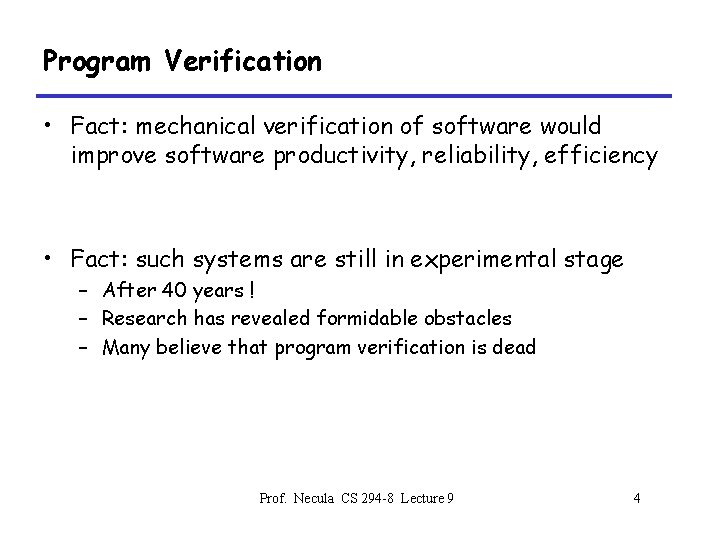
Program Verification • Fact: mechanical verification of software would improve software productivity, reliability, efficiency • Fact: such systems are still in experimental stage – After 40 years ! – Research has revealed formidable obstacles – Many believe that program verification is dead Prof. Necula CS 294 -8 Lecture 9 4

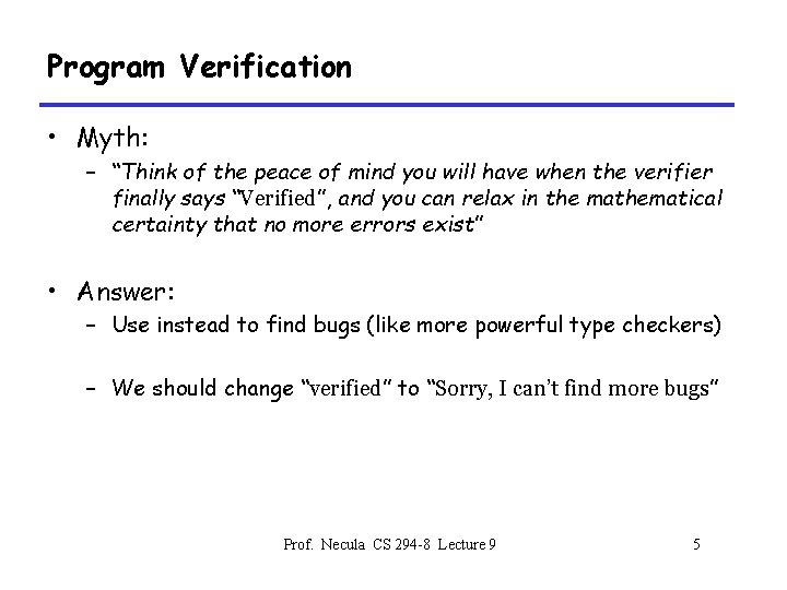
Program Verification • Myth: – “Think of the peace of mind you will have when the verifier finally says “Verified”, and you can relax in the mathematical certainty that no more errors exist” • Answer: – Use instead to find bugs (like more powerful type checkers) – We should change “verified” to “Sorry, I can’t find more bugs” Prof. Necula CS 294 -8 Lecture 9 5

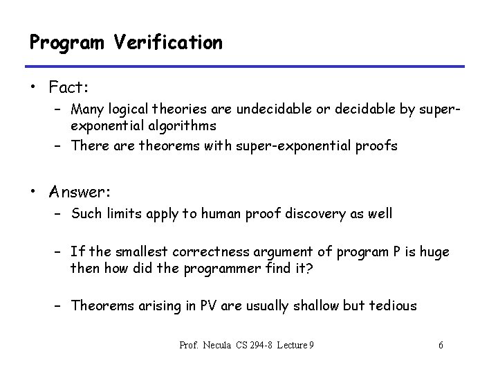
Program Verification • Fact: – Many logical theories are undecidable or decidable by superexponential algorithms – There are theorems with super-exponential proofs • Answer: – Such limits apply to human proof discovery as well – If the smallest correctness argument of program P is huge then how did the programmer find it? – Theorems arising in PV are usually shallow but tedious Prof. Necula CS 294 -8 Lecture 9 6

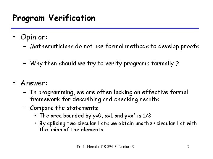
Program Verification • Opinion: – Mathematicians do not use formal methods to develop proofs – Why then should we try to verify programs formally ? • Answer: – In programming, we are often lacking an effective formal framework for describing and checking results – Compare the statements • The area bounded by y=0, x=1 and y=x 2 is 1/3 • By splicing two circular lists we obtain another circular list with the union of the elements Prof. Necula CS 294 -8 Lecture 9 7

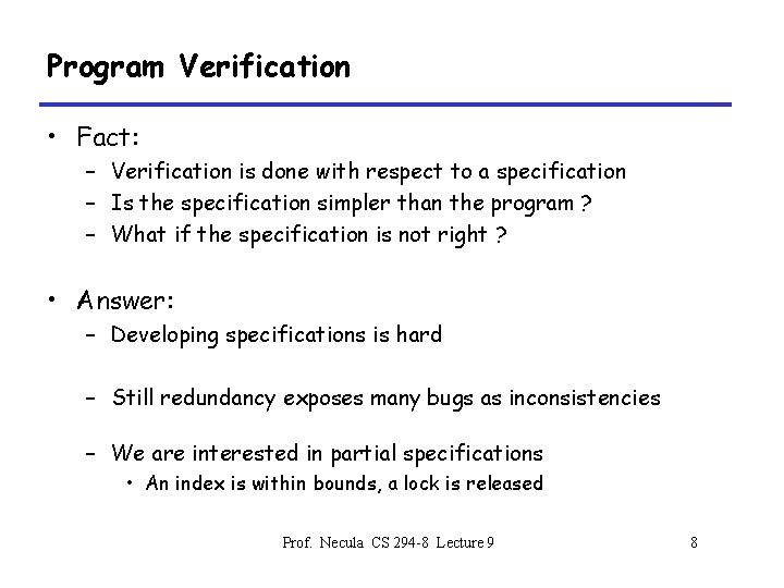
Program Verification • Fact: – Verification is done with respect to a specification – Is the specification simpler than the program ? – What if the specification is not right ? • Answer: – Developing specifications is hard – Still redundancy exposes many bugs as inconsistencies – We are interested in partial specifications • An index is within bounds, a lock is released Prof. Necula CS 294 -8 Lecture 9 8

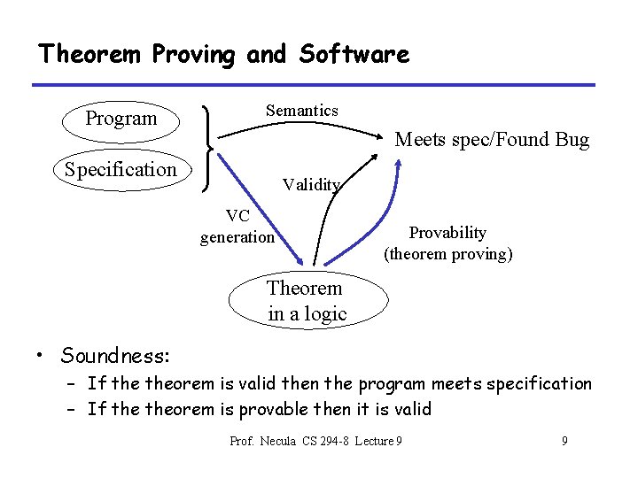
Theorem Proving and Software Program Semantics Meets spec/Found Bug Specification Validity VC generation Provability (theorem proving) Theorem in a logic • Soundness: – If theorem is valid then the program meets specification – If theorem is provable then it is valid Prof. Necula CS 294 -8 Lecture 9 9

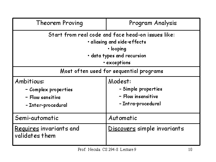
Theorem Proving Program Analysis Start from real code and face head-on issues like: • aliasing and side-effects • looping • data types and recursion • exceptions Most often used for sequential programs Ambitious: Modest: – Simple properties – Complex properties – Flow sensitive – Flow insensitive – Intra-procedural – Inter-procedural Semi-automatic Automatic Requires invariants and validates them Discovers simple invariants Prof. Necula CS 294 -8 Lecture 9 10

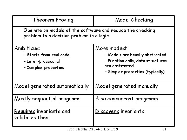
Theorem Proving Model Checking Operate on models of the software and reduce the checking problem to a decision problem in a logic Ambitious: More modest: – Starts from real code – Inter-procedural – Complex properties – Models are heavily abstracted – Function calls, data structures are abstracted – Simpler properties (typically) Model generated automatically Model generated manually Mostly sequential programs Also concurrent programs Requires invariants and validates them Discovers invariants Prof. Necula CS 294 -8 Lecture 9 11

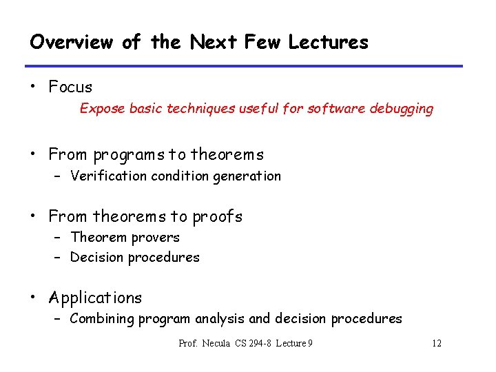
Overview of the Next Few Lectures • Focus Expose basic techniques useful for software debugging • From programs to theorems – Verification condition generation • From theorems to proofs – Theorem provers – Decision procedures • Applications – Combining program analysis and decision procedures Prof. Necula CS 294 -8 Lecture 9 12

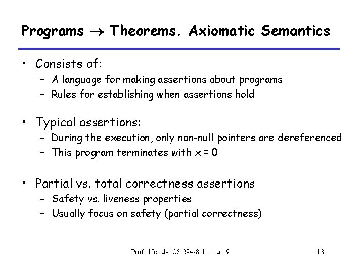
Programs Theorems. Axiomatic Semantics • Consists of: – A language for making assertions about programs – Rules for establishing when assertions hold • Typical assertions: – During the execution, only non-null pointers are dereferenced – This program terminates with x = 0 • Partial vs. total correctness assertions – Safety vs. liveness properties – Usually focus on safety (partial correctness) Prof. Necula CS 294 -8 Lecture 9 13

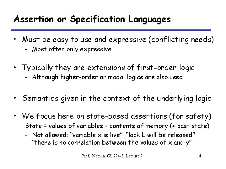
Assertion or Specification Languages • Must be easy to use and expressive (conflicting needs) – Most often only expressive • Typically they are extensions of first-order logic – Although higher-order or modal logics are also used • Semantics given in the context of the underlying logic • We focus here on state-based assertions (for safety) State = values of variables + contents of memory (+ past state) – Not allowed: “variable x is live”, “lock L will be released”, “there is no correlation between the values of x and y” Prof. Necula CS 294 -8 Lecture 9 14

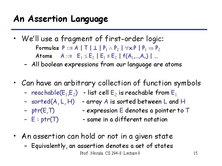
An Assertion Language • We’ll use a fragment of first-order logic: Formulas P : : = A | T | | P 1 P 2 | x. P | P 1 P 2 Atoms A : : = E 1 E 2 | E 1 = E 2 | f(A 1, …, An) | … – All boolean expressions from our language are atoms • Can have an arbitrary collection of function symbols – – reachable(E 1, E 2) sorted(A, L, H) ptr(E, T) E : ptr(T) - list cell E 2 is reachable from E 1 - array A is sorted between L and H - expression E denotes a pointer to T - same in a different notation • An assertion can hold or not in a given state – Equivalently, an assertion denotes a set of states Prof. Necula CS 294 -8 Lecture 9 15

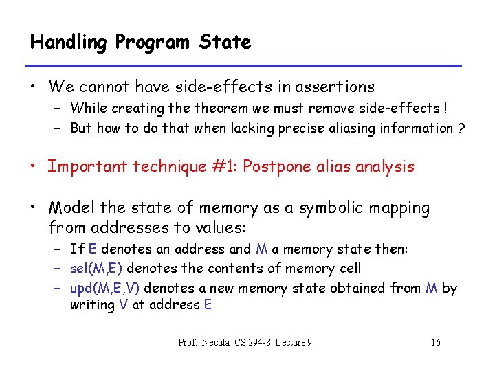
Handling Program State • We cannot have side-effects in assertions – While creating theorem we must remove side-effects ! – But how to do that when lacking precise aliasing information ? • Important technique #1: Postpone alias analysis • Model the state of memory as a symbolic mapping from addresses to values: – If E denotes an address and M a memory state then: – sel(M, E) denotes the contents of memory cell – upd(M, E, V) denotes a new memory state obtained from M by writing V at address E Prof. Necula CS 294 -8 Lecture 9 16

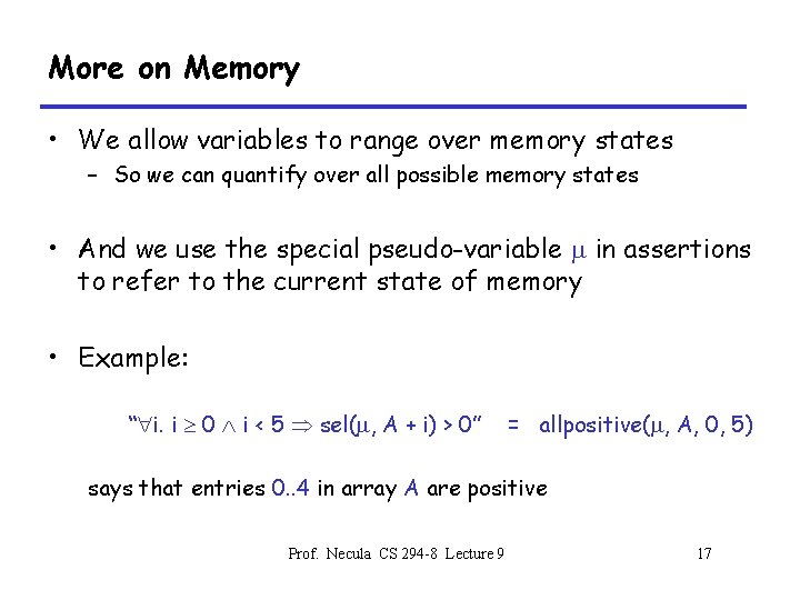
More on Memory • We allow variables to range over memory states – So we can quantify over all possible memory states • And we use the special pseudo-variable in assertions to refer to the current state of memory • Example: “ i. i 0 i < 5 sel( , A + i) > 0” = allpositive( , A, 0, 5) says that entries 0. . 4 in array A are positive Prof. Necula CS 294 -8 Lecture 9 17

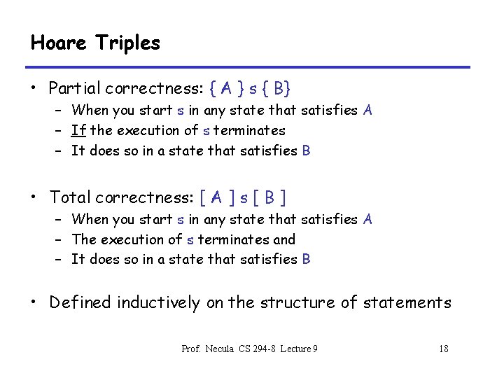
Hoare Triples • Partial correctness: { A } s { B} – When you start s in any state that satisfies A – If the execution of s terminates – It does so in a state that satisfies B • Total correctness: [ A ] s [ B ] – When you start s in any state that satisfies A – The execution of s terminates and – It does so in a state that satisfies B • Defined inductively on the structure of statements Prof. Necula CS 294 -8 Lecture 9 18

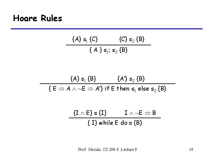
Hoare Rules {A} s 1 {C} s 2 {B} { A } s 1; s 2 {B} {A} s 1 {B} {A’} s 2 {B} { E A’} if E then s 1 else s 2 {B} {I E} s {I} I E B { I} while E do s {B} Prof. Necula CS 294 -8 Lecture 9 19

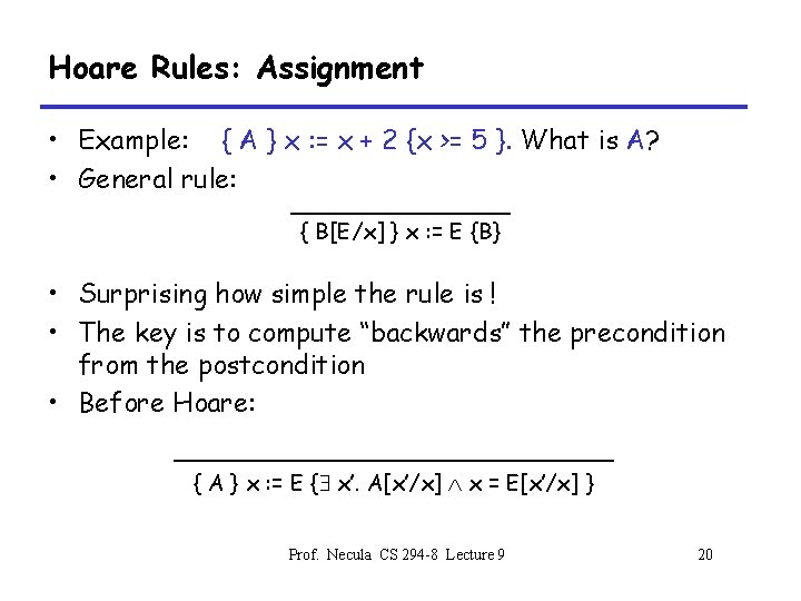
Hoare Rules: Assignment • Example: { A } x : = x + 2 {x >= 5 }. What is A? • General rule: { B[E/x] } x : = E {B} • Surprising how simple the rule is ! • The key is to compute “backwards” the precondition from the postcondition • Before Hoare: { A } x : = E { x’. A[x’/x] x = E[x’/x] } Prof. Necula CS 294 -8 Lecture 9 20

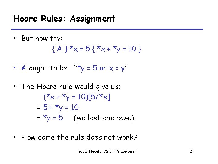
Hoare Rules: Assignment • But now try: { A } *x = 5 { *x + *y = 10 } • A ought to be “*y = 5 or x = y” • The Hoare rule would give us: (*x + *y = 10)[5/*x] = 5 + *y = 10 = *y = 5 (we lost one case) • How come the rule does not work? Prof. Necula CS 294 -8 Lecture 9 21

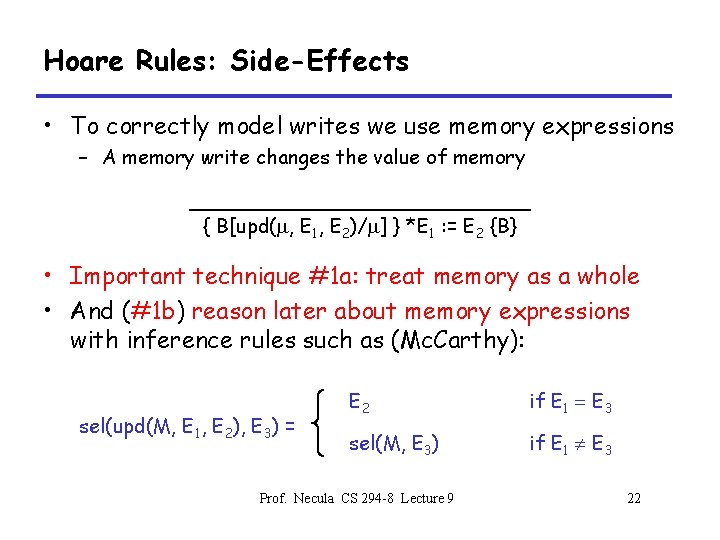
Hoare Rules: Side-Effects • To correctly model writes we use memory expressions – A memory write changes the value of memory { B[upd( , E 1, E 2)/ ] } *E 1 : = E 2 {B} • Important technique #1 a: treat memory as a whole • And (#1 b) reason later about memory expressions with inference rules such as (Mc. Carthy): sel(upd(M, E 1, E 2), E 3) = E 2 if E 1 = E 3 sel(M, E 3) if E 1 ¹ E 3 Prof. Necula CS 294 -8 Lecture 9 22

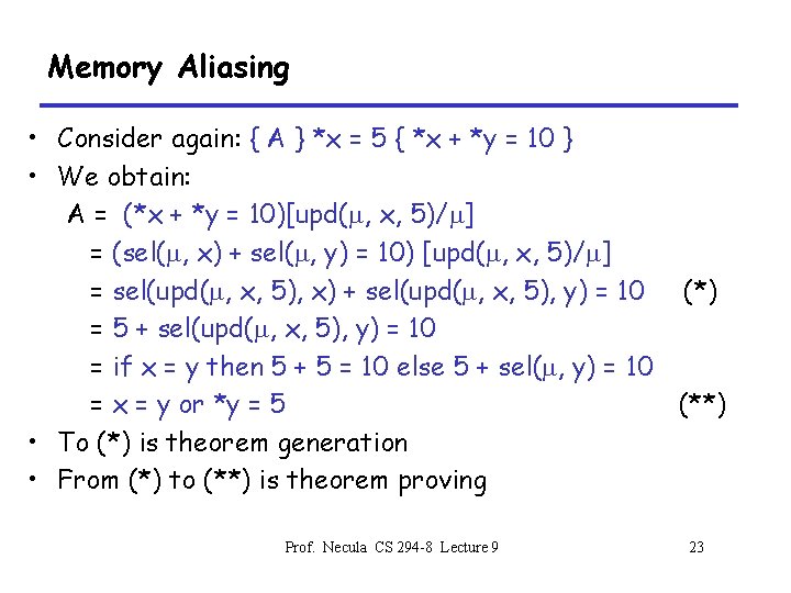
Memory Aliasing • Consider again: { A } *x = 5 { *x + *y = 10 } • We obtain: A = (*x + *y = 10)[upd( , x, 5)/ ] = (sel( , x) + sel( , y) = 10) [upd( , x, 5)/ ] = sel(upd( , x, 5), x) + sel(upd( , x, 5), y) = 10 (*) = 5 + sel(upd( , x, 5), y) = 10 = if x = y then 5 + 5 = 10 else 5 + sel( , y) = 10 = x = y or *y = 5 (**) • To (*) is theorem generation • From (*) to (**) is theorem proving Prof. Necula CS 294 -8 Lecture 9 23

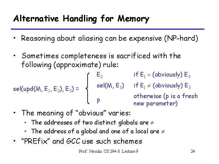
Alternative Handling for Memory • Reasoning about aliasing can be expensive (NP-hard) • Sometimes completeness is sacrificed with the following (approximate) rule: sel(upd(M, E 1, E 2), E 3) = E 2 if E 1 = (obviously) E 3 sel(M, E 3) if E 1 ¹ (obviously) E 3 p otherwise (p is a fresh new parameter) • The meaning of “obvious” varies: • The addresses of two distinct globals are ¹ • The address of a global and one of a local are ¹ • “PREfix” and GCC use such schemes Prof. Necula CS 294 -8 Lecture 9 24

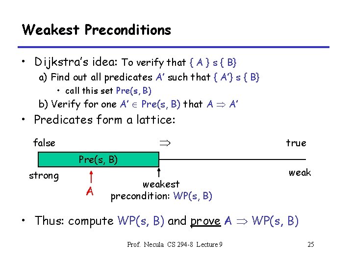
Weakest Preconditions • Dijkstra’s idea: To verify that { A } s { B} a) Find out all predicates A’ such that { A’} s { B} • call this set Pre(s, B) b) Verify for one A’ Pre(s, B) that A A’ • Predicates form a lattice: false Pre(s, B) strong A weakest precondition: WP(s, B) true weak • Thus: compute WP(s, B) and prove A WP(s, B) Prof. Necula CS 294 -8 Lecture 9 25

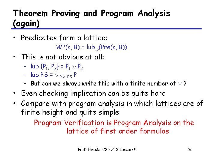
Theorem Proving and Program Analysis (again) • Predicates form a lattice: WP(s, B) = lub (Pre(s, B)) • This is not obvious at all: – lub {P 1, P 2} = P 1 P 2 – lub PS = P PS P – But can we always write this with a finite number of ? • Even checking implication can be quite hard • Compare with program analysis in which lattices are of finite height and quite simple Program Verification is Program Analysis on the lattice of first order formulas Prof. Necula CS 294 -8 Lecture 9 26

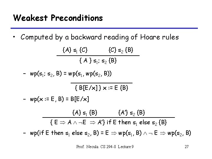
Weakest Preconditions • Computed by a backward reading of Hoare rules {A} s 1 {C} s 2 {B} { A } s 1; s 2 {B} – wp(s 1; s 2, B) = wp(s 1, wp(s 2, B)) { B[E/x] } x : = E {B} – wp(x : = E, B) = B[E/x] {A} s 1 {B} {A’} s 2 {B} { E A’} if E then s 1 else s 2 {B} – wp(if E then s 1 else s 2, B) = E wp(s 1, B) E wp(s 2, B) Prof. Necula CS 294 -8 Lecture 9 27

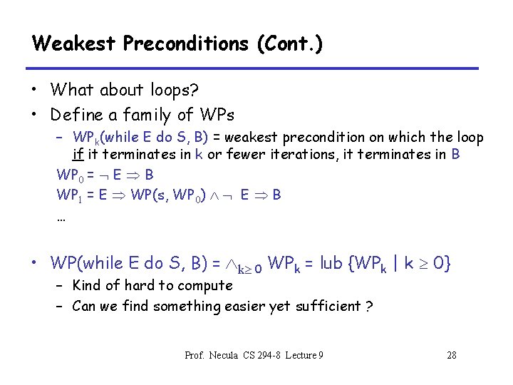
Weakest Preconditions (Cont. ) • What about loops? • Define a family of WPs – WPk(while E do S, B) = weakest precondition on which the loop if it terminates in k or fewer iterations, it terminates in B WP 0 = E B WP 1 = E WP(s, WP 0) E B … • WP(while E do S, B) = k 0 WPk = lub {WPk | k 0} – Kind of hard to compute – Can we find something easier yet sufficient ? Prof. Necula CS 294 -8 Lecture 9 28

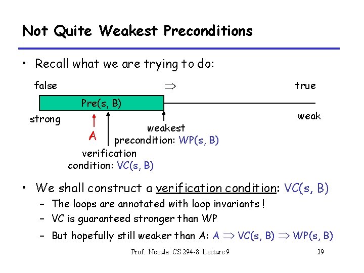
Not Quite Weakest Preconditions • Recall what we are trying to do: false Pre(s, B) strong weakest A precondition: WP(s, B) verification condition: VC(s, B) true weak • We shall construct a verification condition: VC(s, B) – The loops are annotated with loop invariants ! – VC is guaranteed stronger than WP – But hopefully still weaker than A: A VC(s, B) WP(s, B) Prof. Necula CS 294 -8 Lecture 9 29

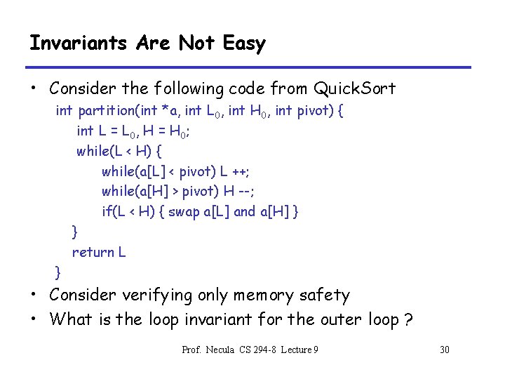
Invariants Are Not Easy • Consider the following code from Quick. Sort int partition(int *a, int L 0, int H 0, int pivot) { int L = L 0, H = H 0; while(L < H) { while(a[L] < pivot) L ++; while(a[H] > pivot) H --; if(L < H) { swap a[L] and a[H] } } return L } • Consider verifying only memory safety • What is the loop invariant for the outer loop ? Prof. Necula CS 294 -8 Lecture 9 30