The PAQ 4 Data Compressor Matt Mahoney Florida

The PAQ 4 Data Compressor Matt Mahoney Florida Tech.

Outline • • Data compression background The PAQ 4 compressor Modeling NASA valve data History of PAQ 4 development

Data Compression Background • • Lossy vs. lossless Theoretical limits on lossless compression Difficulty of modeling data Current compression algorithms

Lossy vs. Lossless • Lossy compression discards unimportant information – NTSC (color TV), JPEG, MPEG discard imperceptible image details – MP 3 discards inaudible details • Losslessly compressed data can be restored exactly

Theoretical Limits on Lossless Compression • Cannot compress random data • Cannot compress recursively • Cannot compress every possible message – Every compression algorithm must expand some messages by at least 1 bit • Cannot compress x better than log 2 1/P(x) bits on average (Shannon, 1949)

Difficulty of Modeling • In general, the probability distribution P of a source is unknown • Estimating P is called modeling • Modeling is hard – Text: as hard as AI – Encrypted data: as hard as cryptanalysis

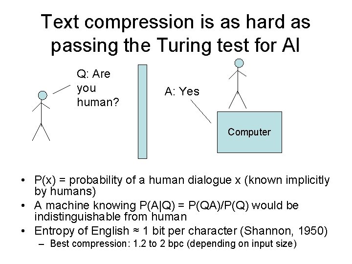
Text compression is as hard as passing the Turing test for AI Q: Are you human? A: Yes Computer • P(x) = probability of a human dialogue x (known implicitly by humans) • A machine knowing P(A|Q) = P(QA)/P(Q) would be indistinguishable from human • Entropy of English ≈ 1 bit per character (Shannon, 1950) – Best compression: 1. 2 to 2 bpc (depending on input size)

Compressing encrypted data is equivalent to breaking the encryption • Example: x = 1, 000 0 bytes encrypted with AES in CBC mode and key “foobar” • The encrypted data passes all tests for statistical randomness (not compressible) • C(x) = 65 bytes using English • Finding C(x) requires guessing the key

Nevertheless, some common data is compressible

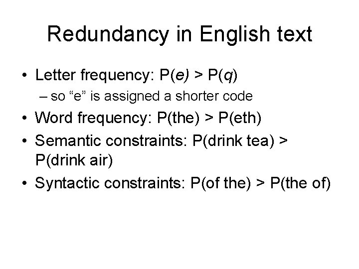
Redundancy in English text • Letter frequency: P(e) > P(q) – so “e” is assigned a shorter code • Word frequency: P(the) > P(eth) • Semantic constraints: P(drink tea) > P(drink air) • Syntactic constraints: P(of the) > P(the of)

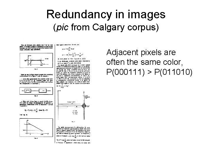
Redundancy in images (pic from Calgary corpus) Adjacent pixels are often the same color, P(000111) > P(011010)

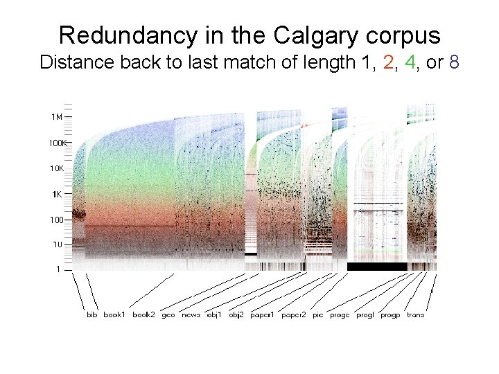
Redundancy in the Calgary corpus Distance back to last match of length 1, 2, 4, or 8

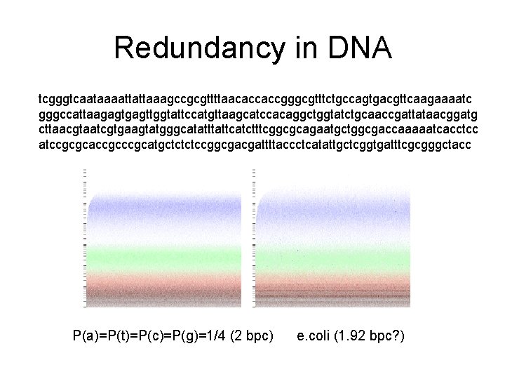
Redundancy in DNA tcgggtcaataaaattattaaagccgcgttttaacaccaccgggcgtttctgccagtgacgttcaagaaaatc gggccattaagagttggtattccatgttaagcatccacaggctggtatctgcaaccgattataacggatg cttaacgtaatcgtgaagtatgggcatattcatctttcggcgcagaatgctggcgaccaaaaatcacctcc atccgcgcaccgcatgctctctccggcgacgattttaccctcatattgctcggtgatttcgcgggctacc P(a)=P(t)=P(c)=P(g)=1/4 (2 bpc) e. coli (1. 92 bpc? )

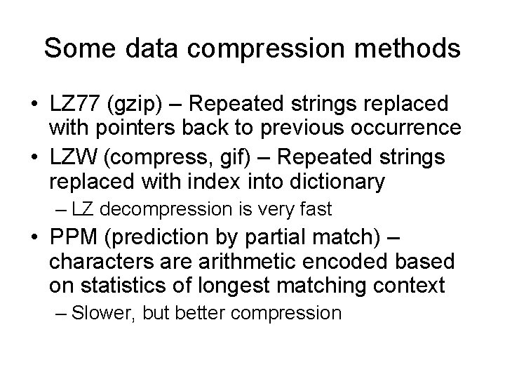
Some data compression methods • LZ 77 (gzip) – Repeated strings replaced with pointers back to previous occurrence • LZW (compress, gif) – Repeated strings replaced with index into dictionary – LZ decompression is very fast • PPM (prediction by partial match) – characters are arithmetic encoded based on statistics of longest matching context – Slower, but better compression

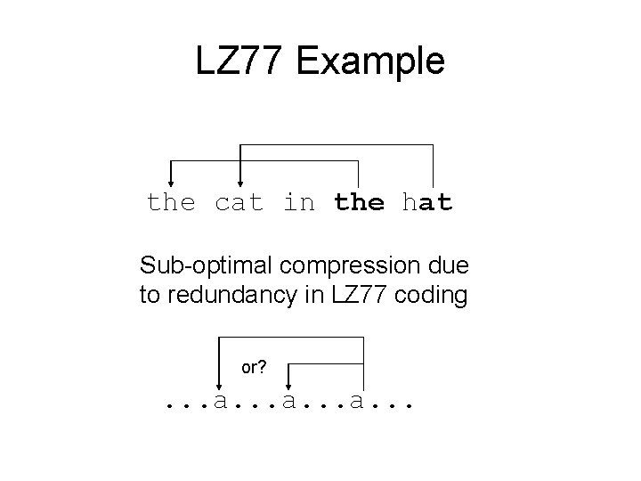
LZ 77 Example the cat in the hat Sub-optimal compression due to redundancy in LZ 77 coding or? . . . a. . .

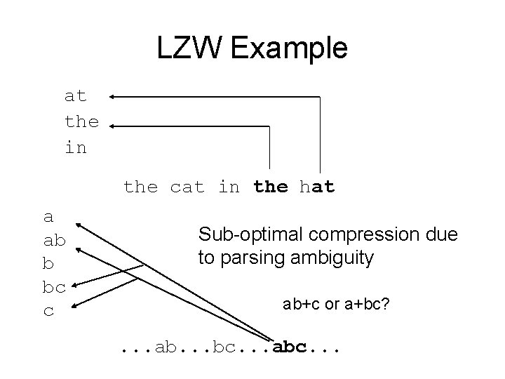
LZW Example at the in the cat in the hat a ab b bc c Sub-optimal compression due to parsing ambiguity ab+c or a+bc? . . . ab. . . bc. . . abc. . .

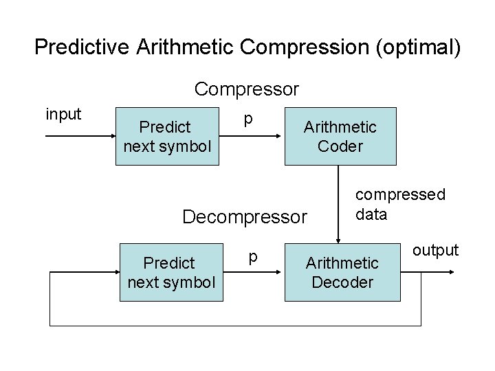
Predictive Arithmetic Compression (optimal) Compressor input Predict next symbol p Arithmetic Coder Decompressor Predict next symbol p compressed data Arithmetic Decoder output

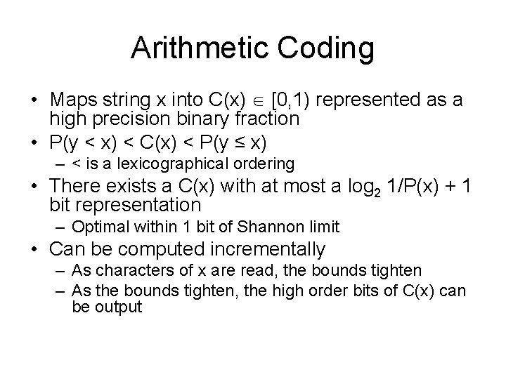
Arithmetic Coding • Maps string x into C(x) [0, 1) represented as a high precision binary fraction • P(y < x) < C(x) < P(y ≤ x) – < is a lexicographical ordering • There exists a C(x) with at most a log 2 1/P(x) + 1 bit representation – Optimal within 1 bit of Shannon limit • Can be computed incrementally – As characters of x are read, the bounds tighten – As the bounds tighten, the high order bits of C(x) can be output

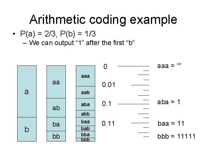
Arithmetic coding example • P(a) = 2/3, P(b) = 1/3 – We can output “ 1” after the first “b” 0 aa a b aaa = “” aaa 0. 01 aab ab aba ba bab bba bbb bb 0. 1 aba = 1 0. 11 baa = 11 abb bbb = 11111

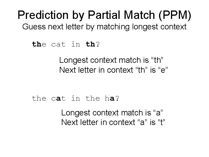
Prediction by Partial Match (PPM) Guess next letter by matching longest context the cat in th? Longest context match is “th” Next letter in context “th” is “e” the cat in the ha? Longest context match is “a” Next letter in context “a” is “t”

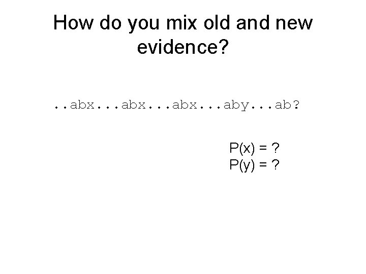
How do you mix old and new evidence? . . abx. . . aby. . . ab? P(x) = ? P(y) = ?

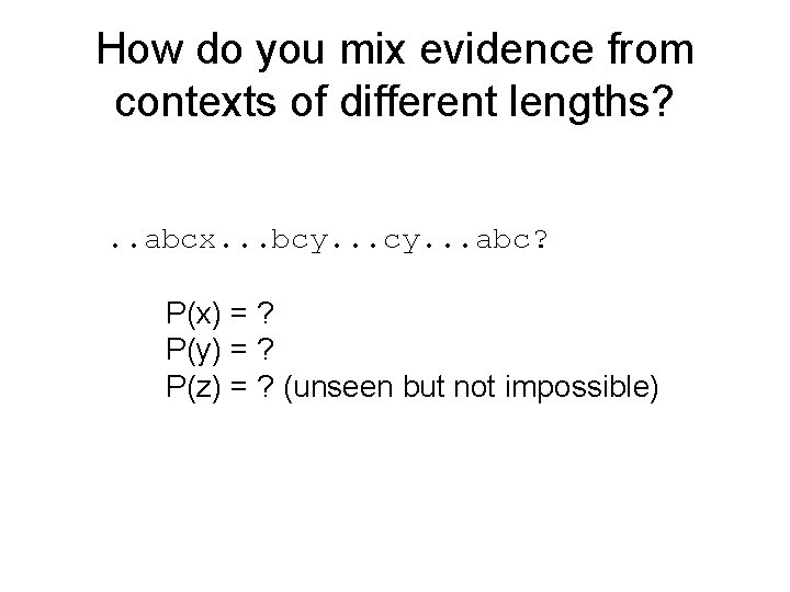
How do you mix evidence from contexts of different lengths? . . abcx. . . bcy. . . abc? P(x) = ? P(y) = ? P(z) = ? (unseen but not impossible)

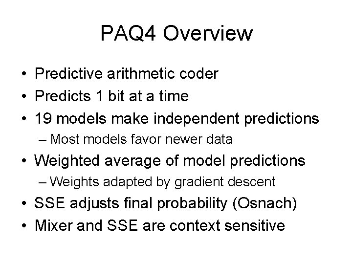
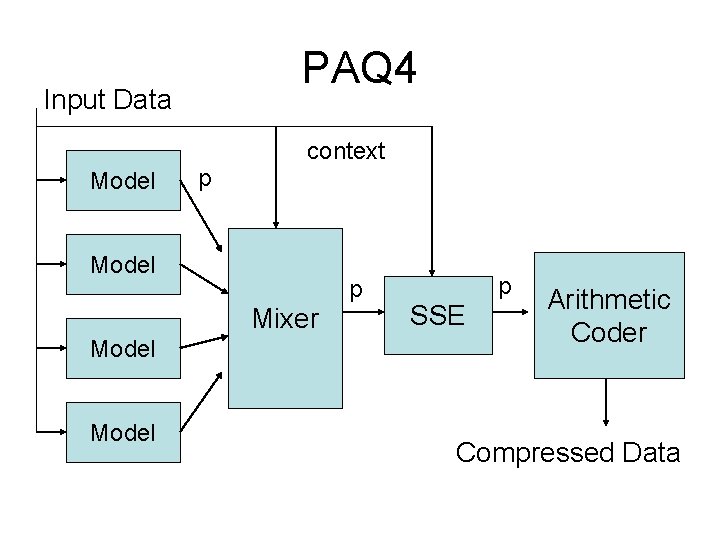
PAQ 4 Overview • Predictive arithmetic coder • Predicts 1 bit at a time • 19 models make independent predictions – Most models favor newer data • Weighted average of model predictions – Weights adapted by gradient descent • SSE adjusts final probability (Osnach) • Mixer and SSE are context sensitive

PAQ 4 Input Data context Model p Mixer Model p SSE Arithmetic Coder Compressed Data

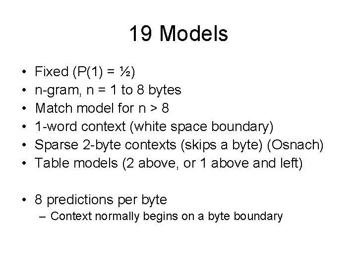
19 Models • • • Fixed (P(1) = ½) n-gram, n = 1 to 8 bytes Match model for n > 8 1 -word context (white space boundary) Sparse 2 -byte contexts (skips a byte) (Osnach) Table models (2 above, or 1 above and left) • 8 predictions per byte – Context normally begins on a byte boundary

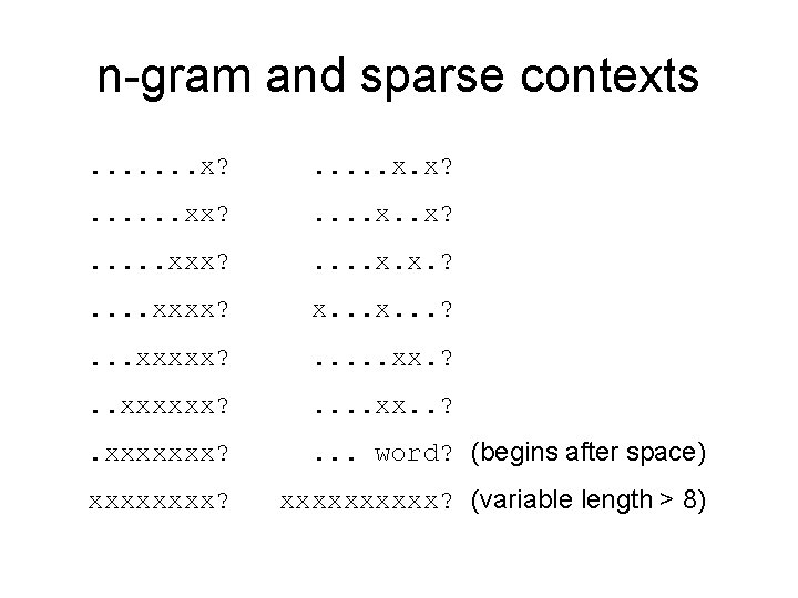
n-gram and sparse contexts. . . . x? . . . xx? . . x? . . . xxx? . . x. x. ? . . xxxx? x. . . ? . . . xxxxx? . . . xx. ? . . xxxxxx? . . xx. . ? . xxxxxxx? . . . word? (begins after space) xxxx? xxxxx? (variable length > 8)

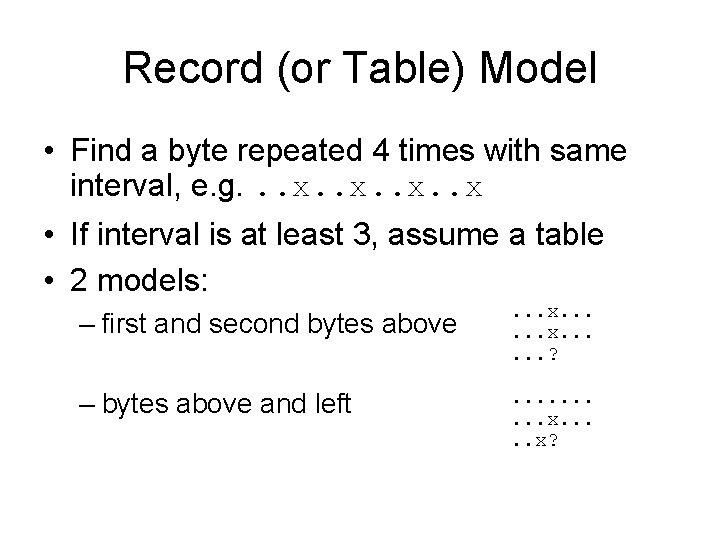
Record (or Table) Model • Find a byte repeated 4 times with same interval, e. g. . . x • If interval is at least 3, assume a table • 2 models: – first and second bytes above . . . x. . . ? – bytes above and left . . x?

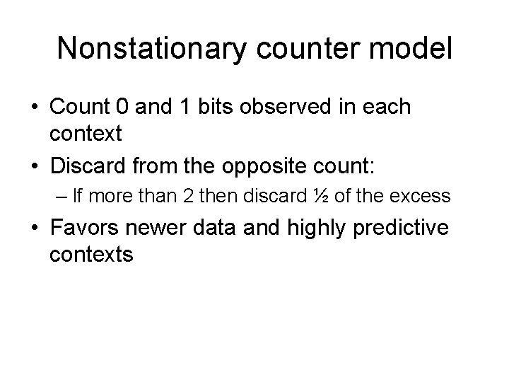
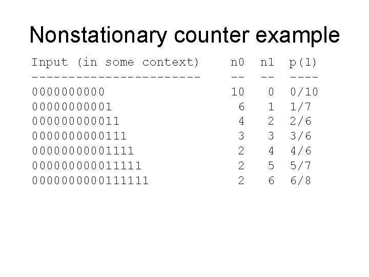
Nonstationary counter model • Count 0 and 1 bits observed in each context • Discard from the opposite count: – If more than 2 then discard ½ of the excess • Favors newer data and highly predictive contexts

Nonstationary counter example Input (in some context) -----------000000000011 0000000000111111 n 0 -10 6 4 3 2 2 2 n 1 -0 1 2 3 4 5 6 p(1) ---0/10 1/7 2/6 3/6 4/6 5/7 6/8

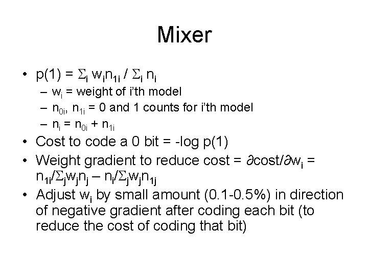
Mixer • p(1) = i win 1 i / i ni – wi = weight of i’th model – n 0 i, n 1 i = 0 and 1 counts for i’th model – ni = n 0 i + n 1 i • Cost to code a 0 bit = -log p(1) • Weight gradient to reduce cost = ∂cost/∂wi = n 1 i/ jwjnj – ni/ jwjn 1 j • Adjust wi by small amount (0. 1 -0. 5%) in direction of negative gradient after coding each bit (to reduce the cost of coding that bit)

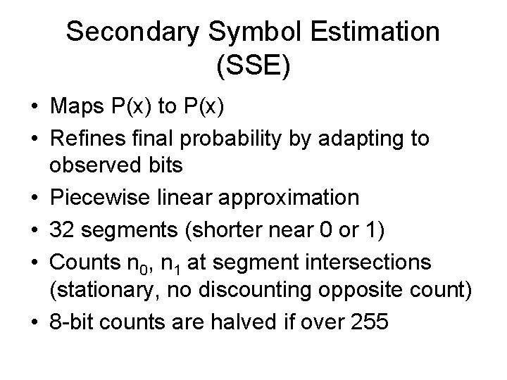
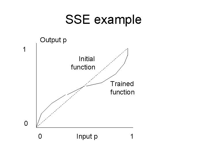
Secondary Symbol Estimation (SSE) • Maps P(x) to P(x) • Refines final probability by adapting to observed bits • Piecewise linear approximation • 32 segments (shorter near 0 or 1) • Counts n 0, n 1 at segment intersections (stationary, no discounting opposite count) • 8 -bit counts are halved if over 255

SSE example Output p 1 Initial function Trained function 0 0 Input p 1

Mixer and SSE are context sensitive • 8 mixers selected by 3 high order bits of last whole byte • 1024 SSE functions selected by current partial byte and 2 high order bits of last whole byte

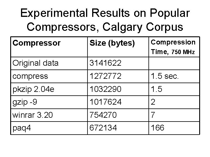
Experimental Results on Popular Compressors, Calgary Corpus Compression Time, 750 MHz Compressor Size (bytes) Original data 3141622 compress 1272772 1. 5 sec. pkzip 2. 04 e 1032290 1. 5 gzip -9 1017624 2 winrar 3. 20 754270 7 paq 4 672134 166

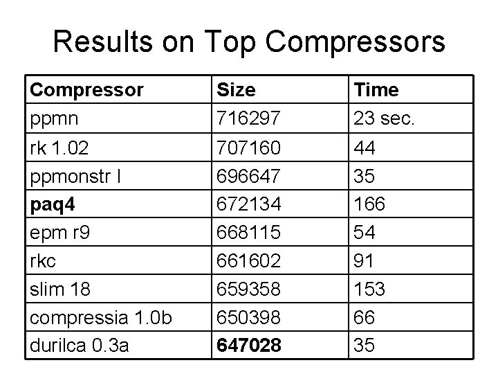
Results on Top Compressors Compressor ppmn Size 716297 Time 23 sec. rk 1. 02 ppmonstr I paq 4 epm r 9 rkc slim 18 compressia 1. 0 b durilca 0. 3 a 707160 696647 672134 668115 661602 659358 650398 647028 44 35 166 54 91 153 66 35

Compression for Anomaly Detection • Anomaly detection: finding unlikely events • Depends on ability to estimate probability • So does compression

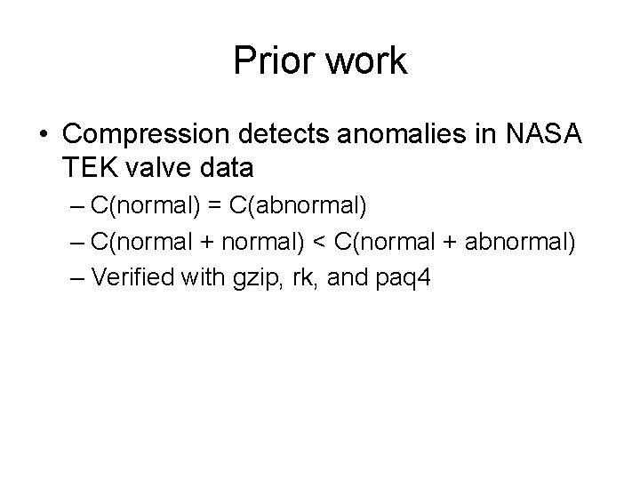
Prior work • Compression detects anomalies in NASA TEK valve data – C(normal) = C(abnormal) – C(normal + normal) < C(normal + abnormal) – Verified with gzip, rk, and paq 4

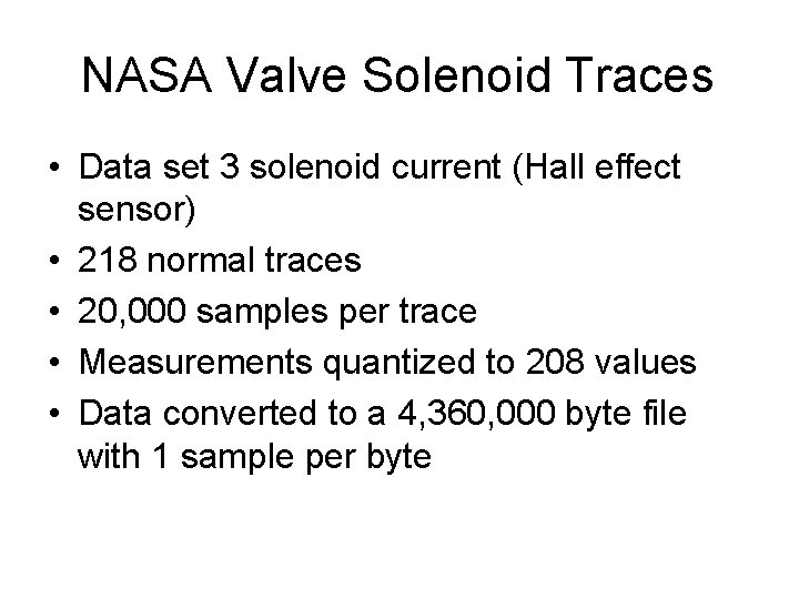
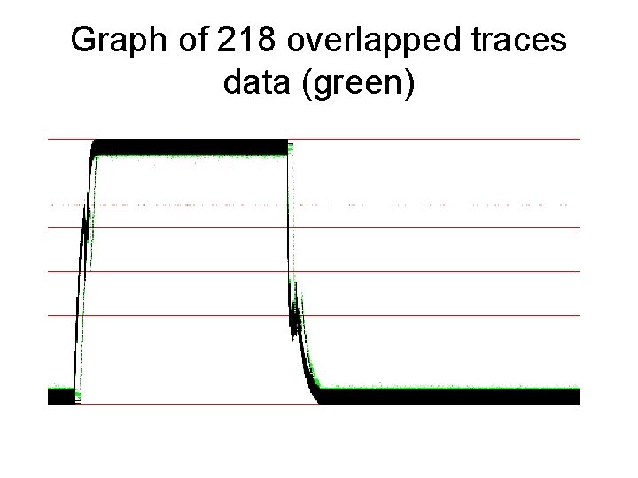
NASA Valve Solenoid Traces • Data set 3 solenoid current (Hall effect sensor) • 218 normal traces • 20, 000 samples per trace • Measurements quantized to 208 values • Data converted to a 4, 360, 000 byte file with 1 sample per byte

Graph of 218 overlapped traces data (green)

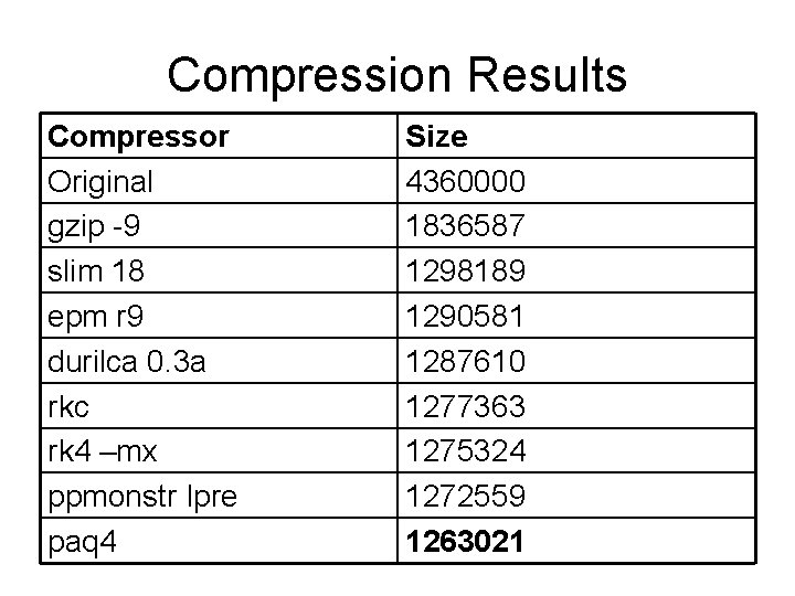
Compression Results Compressor Original gzip -9 slim 18 epm r 9 durilca 0. 3 a rkc rk 4 –mx ppmonstr Ipre paq 4 Size 4360000 1836587 1298189 1290581 1287610 1277363 1275324 1272559 1263021

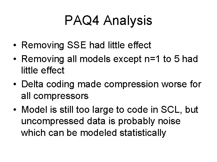
PAQ 4 Analysis • Removing SSE had little effect • Removing all models except n=1 to 5 had little effect • Delta coding made compression worse for all compressors • Model is still too large to code in SCL, but uncompressed data is probably noise which can be modeled statistically

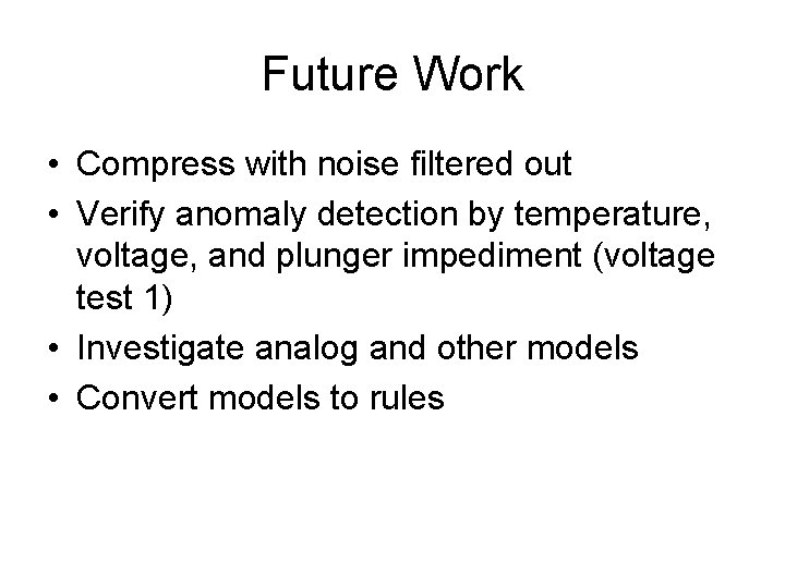
Future Work • Compress with noise filtered out • Verify anomaly detection by temperature, voltage, and plunger impediment (voltage test 1) • Investigate analog and other models • Convert models to rules

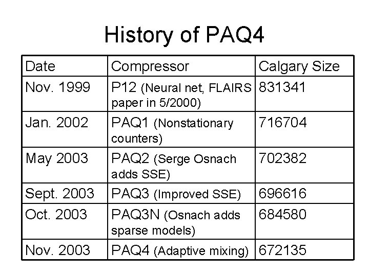
History of PAQ 4 Date Nov. 1999 Compressor Calgary Size P 12 (Neural net, FLAIRS 831341 paper in 5/2000) Jan. 2002 PAQ 1 (Nonstationary 716704 counters) May 2003 PAQ 2 (Serge Osnach 702382 adds SSE) Sept. 2003 Oct. 2003 PAQ 3 (Improved SSE) PAQ 3 N (Osnach adds 696616 684580 sparse models) Nov. 2003 PAQ 4 (Adaptive mixing) 672135

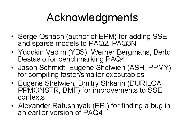
Acknowledgments • Serge Osnach (author of EPM) for adding SSE and sparse models to PAQ 2, PAQ 3 N • Yoockin Vadim (YBS), Werner Bergmans, Berto Destasio for benchmarking PAQ 4 • Jason Schmidt, Eugene Shelwien (ASH, PPMY) for compiling faster/smaller executables • Eugene Shelwien, Dmitry Shkarin (DURILCA, PPMONSTR, BMF) for improvements to SSE contexts • Alexander Ratushnyak (ERI) for finding a bug in an earlier version of PAQ 4