Testing Hypothesis Nutan S Mishra Department of Mathematics

Testing Hypothesis Nutan S. Mishra Department of Mathematics and Statistics University of South Alabama

Description of the problem The population parameter(s) is unknown. Some one (say person A) has some claim about the value of this unknown parameter. Another person (say person B) wants to test how valid is this claim. The person B collects a sample and gathers sample data And proceeds to test the claim.

Example Manufacturer of certain cereal claims that his boxes contain 16 oz on the average. He does not know the true average. He could claim this because he has set up the filling machines to pour 16 oz of material. A consumer protection agency received multiple complaints over a period of time that this brand of boxes contain less amount then claimed. So the consumer protection agency wants to test the claim of the manufacturer. To start with consumer protection agency thinks that on the average boxes contain less than 16 oz.

Example 1 So there are two parties who claim differently about the population parameter. The Manufacturer says average = 16 oz This a prevailing claim in the market. The Consumer Protection Agency says the average is less than 16 oz. This is the doubt raised by the consumer so its consumer protection agency’s responsibility to prove the claim. The consumer protection agency proceeds to test the validity of the claims.

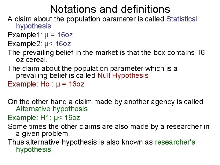
Notations and definitions A claim about the population parameter is called Statistical hypothesis Example 1: µ = 16 oz Example 2: µ< 16 oz The prevailing belief in the market is that the box contains 16 oz cereal. The claim about the population parameter which is a prevailing belief is called Null Hypothesis Example: Ho : µ = 16 oz On the other hand a claim made by another agency is called Alternative hypothesis Example: H 1: µ< 16 oz Some times the other claims are also made by a researcher in a given problem. Thus alternative hypothesis is also known as researcher’s hypothesis.

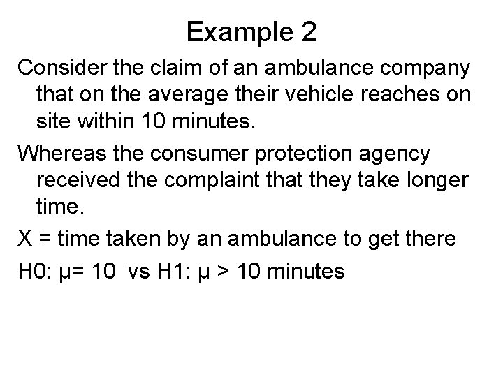
Example 2 Consider the claim of an ambulance company that on the average their vehicle reaches on site within 10 minutes. Whereas the consumer protection agency received the complaint that they take longer time. X = time taken by an ambulance to get there H 0: µ= 10 vs H 1: µ > 10 minutes

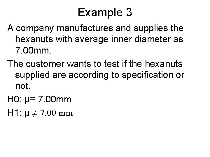
Example 3 A company manufactures and supplies the hexanuts with average inner diameter as 7. 00 mm. The customer wants to test if the hexanuts supplied are according to specification or not. H 0: µ= 7. 00 mm H 1: µ ≠ 7. 00 mm

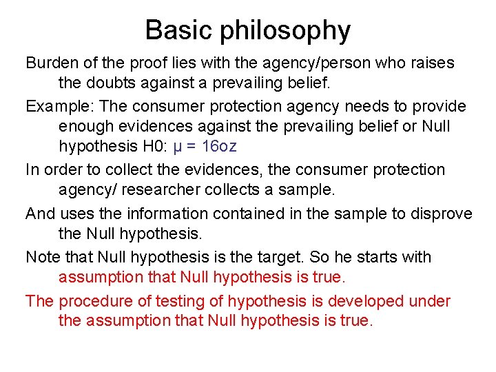
Basic philosophy Burden of the proof lies with the agency/person who raises the doubts against a prevailing belief. Example: The consumer protection agency needs to provide enough evidences against the prevailing belief or Null hypothesis H 0: µ = 16 oz In order to collect the evidences, the consumer protection agency/ researcher collects a sample. And uses the information contained in the sample to disprove the Null hypothesis. Note that Null hypothesis is the target. So he starts with assumption that Null hypothesis is true. The procedure of testing of hypothesis is developed under the assumption that Null hypothesis is true.

Definitions A null hypothesis is a claim about the population parameter that is assumed to be true until it is declared to be false. An alternative hypothesis is a claim about population parameter that will be true if null hypothesis is false.

Method for population mean • • • Step 1 : define null and alternative hypotheses. Step 2 : Collect a sample of size n Step 3 : Compute the sample mean. Step 4: compare the sample mean with the critical value Recall that if we collect different samples, value of the sample mean will be different. And there is always a difference between sample mean and population mean This difference occurs due to: – Sampling errors (chance errors which are inherent) – Non sampling errors ( due to some assignable cause) If the difference is too big, its easy to make a decision on H 0. When the difference is small we need to analyze it carefully. We want to find out whether the difference in sample mean and claimed value of population mean has occurred just due to chance or is there any systematic cause behind this difference?

Method for population mean • • Step 1 : define null and alternative hypotheses. Step 2 : Collect a sample of size n Step 3 : Compute the sample mean. Step 4: compare the sample mean with the critical value Question: How to find the critical value? To find the critical value we need to take into account two types of errors which may incur in our decision.

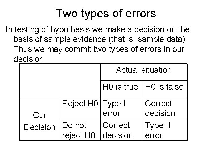
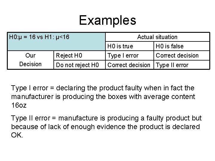
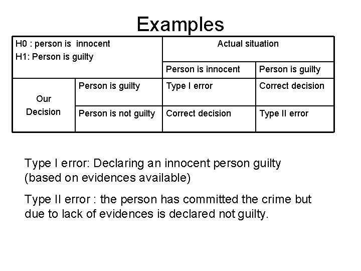
Two types of errors In testing of hypothesis we make a decision on the basis of sample evidence (that is sample data). Thus we may commit two types of errors in our decision Actual situation H 0 is true H 0 is false Reject H 0 Type I error Our Correct Decision Do not reject H 0 decision Correct decision Type II error

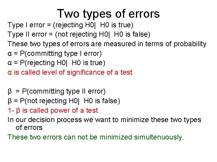
Two types of errors Type I error = (rejecting H 0| H 0 is true) Type II error = (not rejecting H 0| H 0 is false) These two types of errors are measured in terms of probability α = P(committing type I error) α = P(rejecting H 0| H 0 is true) α is called level of significance of a test β = P(committing type II error) β = P(not rejecting H 0| H 0 is false) 1 - β is called power of a test In our decision process we want to minimize these two types of errors These two errors can not be minimized simultenuously.

Examples H 0: µ = 16 vs H 1: µ<16 Our Decision Actual situation H 0 is true H 0 is false Reject H 0 Type I error Correct decision Do not reject H 0 Correct decision Type II error Type I error = declaring the product faulty when in fact the manufacturer is producing the boxes with average content 16 oz Type II error = manufacture is producing a faulty product but because of lack of enough evidence the product is declared OK.

Examples H 0 : person is innocent H 1: Person is guilty Our Decision Actual situation Person is innocent Person is guilty Type I error Correct decision Person is not guilty Correct decision Type II error Type I error: Declaring an innocent person guilty (based on evidences available) Type II error : the person has committed the crime but due to lack of evidences is declared not guilty.

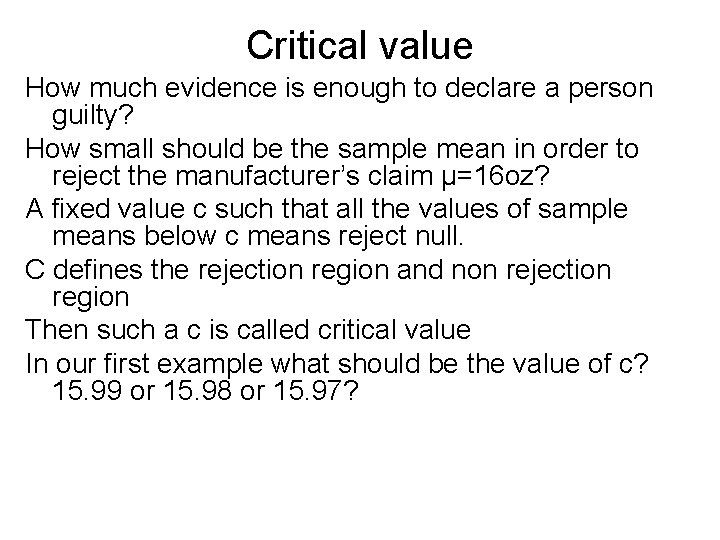
Critical value How much evidence is enough to declare a person guilty? How small should be the sample mean in order to reject the manufacturer’s claim µ=16 oz? A fixed value c such that all the values of sample means below c means reject null. C defines the rejection region and non rejection region Then such a c is called critical value In our first example what should be the value of c? 15. 99 or 15. 98 or 15. 97?

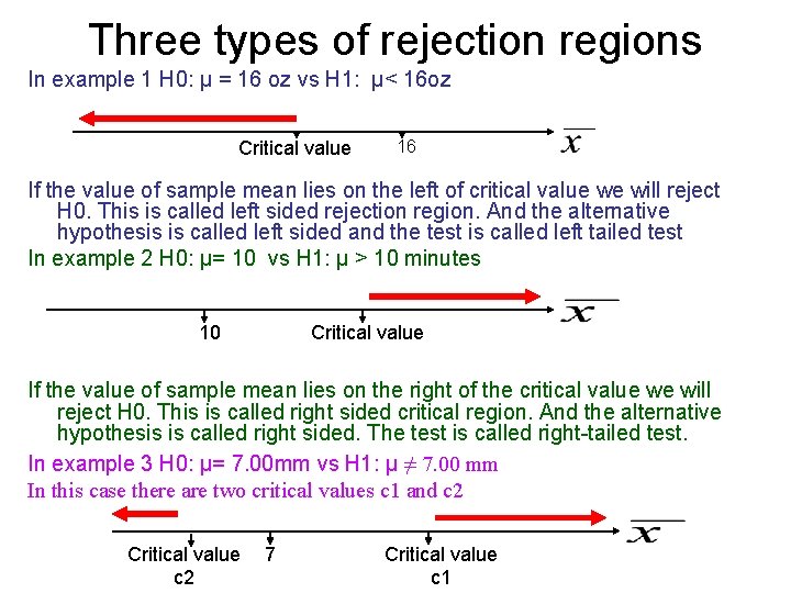
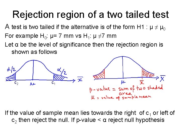
Three types of rejection regions In example 1 H 0: µ = 16 oz vs H 1: µ< 16 oz Critical value 16 If the value of sample mean lies on the left of critical value we will reject H 0. This is called left sided rejection region. And the alternative hypothesis is called left sided and the test is called left tailed test In example 2 H 0: µ= 10 vs H 1: µ > 10 minutes 10 Critical value If the value of sample mean lies on the right of the critical value we will reject H 0. This is called right sided critical region. And the alternative hypothesis is called right sided. The test is called right-tailed test. In example 3 H 0: µ= 7. 00 mm vs H 1: µ ≠ 7. 00 mm In this case there are two critical values c 1 and c 2 Critical value c 2 7 Critical value c 1

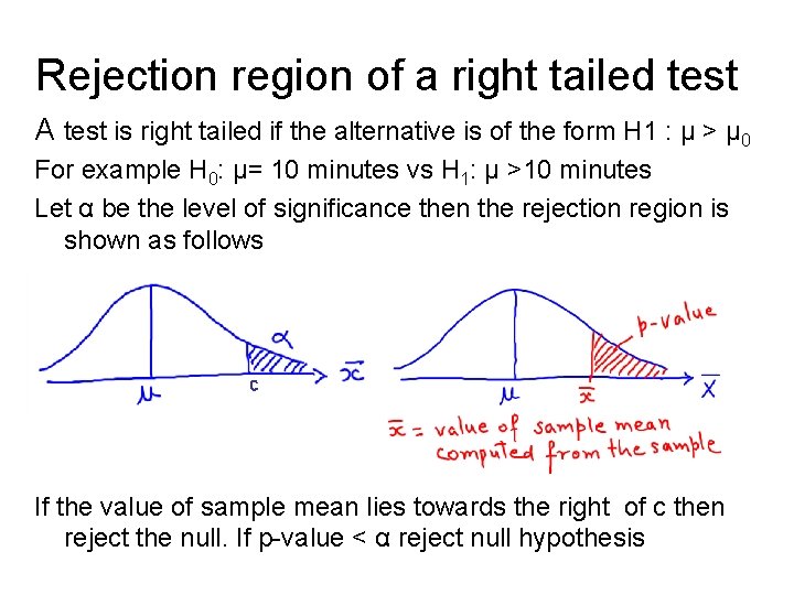
Tails of a test When the alternative hypothesis is of the type µ ≠ µ 0 then the test is called two tailed test because the rejection region lies at the left tail as well as right tail of the distribution of the mean. When alternative hypothesis is of the type µ > µ 0 , then the test is right tailed test because the rejection region lies on the right side of the critical value, that is on the right tail of the curve of sample mean. When alternative is of the type µ < µ 0, then the test is left tailed test because the rejection region lies on the left side of the critical value, that is on the left tail of the curve of sample mean.

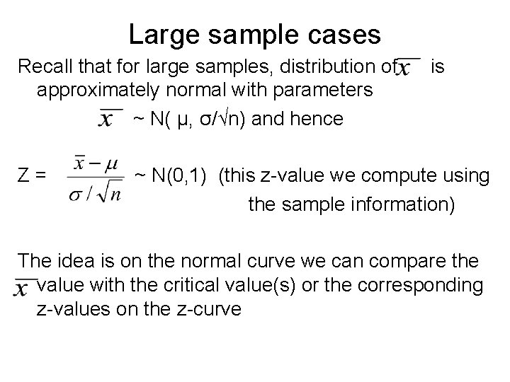
Large sample cases Recall that for large samples, distribution of approximately normal with parameters ~ N( µ, σ/√n) and hence Z= is ~ N(0, 1) (this z-value we compute using the sample information) The idea is on the normal curve we can compare the value with the critical value(s) or the corresponding z-values on the z-curve

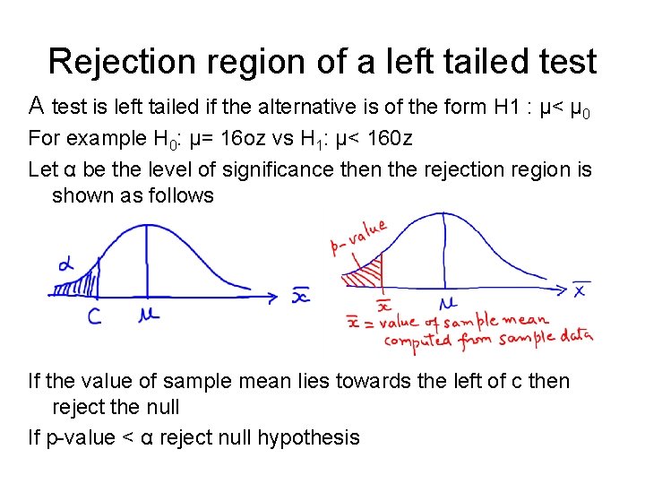
Rejection region of a left tailed test A test is left tailed if the alternative is of the form H 1 : µ< µ 0 For example H 0: µ= 16 oz vs H 1: µ< 160 z Let α be the level of significance then the rejection region is shown as follows If the value of sample mean lies towards the left of c then reject the null If p-value < α reject null hypothesis

Rejection region of a right tailed test A test is right tailed if the alternative is of the form H 1 : µ > µ 0 For example H 0: µ= 10 minutes vs H 1: µ >10 minutes Let α be the level of significance then the rejection region is shown as follows c If the value of sample mean lies towards the right of c then reject the null. If p-value < α reject null hypothesis

Rejection region of a two tailed test A test is two tailed if the alternative is of the form H 1 : µ ≠ µ 0 For example H 0: µ= 7 mm vs H 1: µ ≠ 7 mm Let α be the level of significance then the rejection region is shown as follows c 2 c 1 If the value of sample mean lies towards the right of c 1 or left of c 2 then reject the null. If p-value < α reject null hypothesis

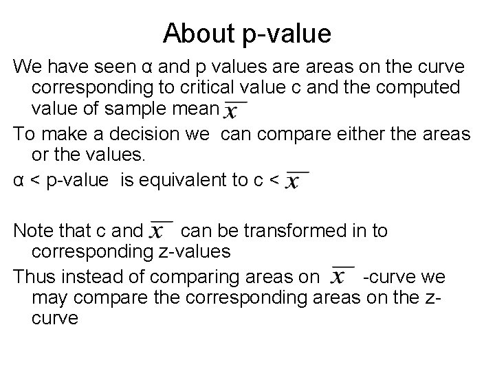
About p-value We have seen α and p values areas on the curve corresponding to critical value c and the computed value of sample mean To make a decision we can compare either the areas or the values. α < p-value is equivalent to c < Note that c and can be transformed in to corresponding z-values Thus instead of comparing areas on -curve we may compare the corresponding areas on the zcurve

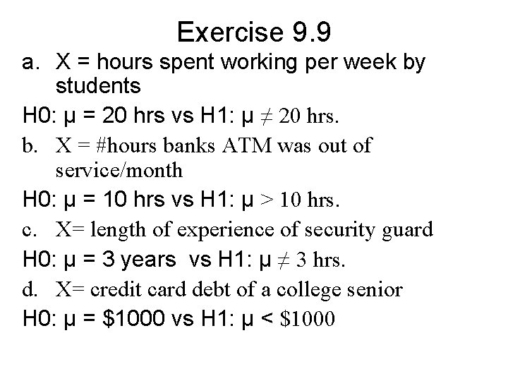
Exercise 9. 9 a. X = hours spent working per week by students H 0: µ = 20 hrs vs H 1: µ ≠ 20 hrs. b. X = #hours banks ATM was out of service/month H 0: µ = 10 hrs vs H 1: µ > 10 hrs. c. X= length of experience of security guard H 0: µ = 3 years vs H 1: µ ≠ 3 hrs. d. X= credit card debt of a college senior H 0: µ = $1000 vs H 1: µ < $1000