Chapter 3 continued Nutan S Mishra Exercises 3

Chapter 3 (continued) Nutan S. Mishra

Exercises 3. 11 -3. 15 • • Size of the data set = 12 for all the five problems In 3. 11 variable x 1 = monthly rent of an apartment ($) In 3. 12 variable x 2 = monthly phone bill ($) In 3. 13 variable x 3 = price of gasoline ($/gallon) In 3. 14 variable x 4 = amount paid to doctor ($/month) In 3. 15 variable x 5 = prices of beer in a city ($) More description of the variables is given on page 82 Since all these five variables describe the amount of money, they are all continuous variables. They may take values between 0 to infinity.

Note Most of the statistical software including minitab prefer the raw (ungrouped) data as input and not the grouped data.

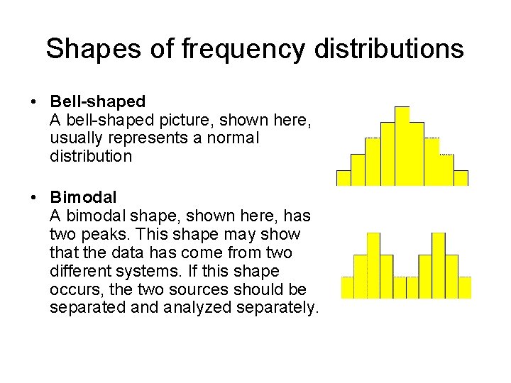
Shapes of frequency distributions • Bell-shaped A bell-shaped picture, shown here, usually represents a normal distribution • Bimodal A bimodal shape, shown here, has two peaks. This shape may show that the data has come from two different systems. If this shape occurs, the two sources should be separated analyzed separately.

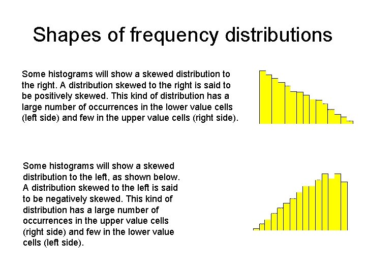
Shapes of frequency distributions Some histograms will show a skewed distribution to the right. A distribution skewed to the right is said to be positively skewed. This kind of distribution has a large number of occurrences in the lower value cells (left side) and few in the upper value cells (right side). Some histograms will show a skewed distribution to the left, as shown below. A distribution skewed to the left is said to be negatively skewed. This kind of distribution has a large number of occurrences in the upper value cells (right side) and few in the lower value cells (left side).

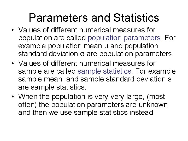
Parameters and Statistics • Values of different numerical measures for population are called population parameters. For example population mean µ and population standard deviation σ are population parameters • Values of different numerical measures for sample are called sample statistics. For example sample mean and sample standard deviation s are sample statistics. • When the population is very large, (most often) the population parameters are unknown and then we use sample statistics instead.

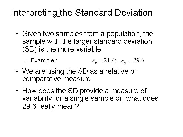
Interpreting the Standard Deviation • Given two samples from a population, the sample with the larger standard deviation (SD) is the more variable – Example : • We are using the SD as a relative or comparative measure • How does the SD provide a measure of variability for a single sample or, what does 29. 6 really mean?

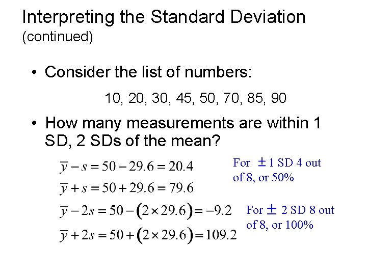
Interpreting the Standard Deviation (continued) • Consider the list of numbers: 10, 20, 30, 45, 50, 70, 85, 90 • How many measurements are within 1 SD, 2 SDs of the mean? For 1 SD 4 out of 8, or 50% For 2 SD 8 out of 8, or 100%

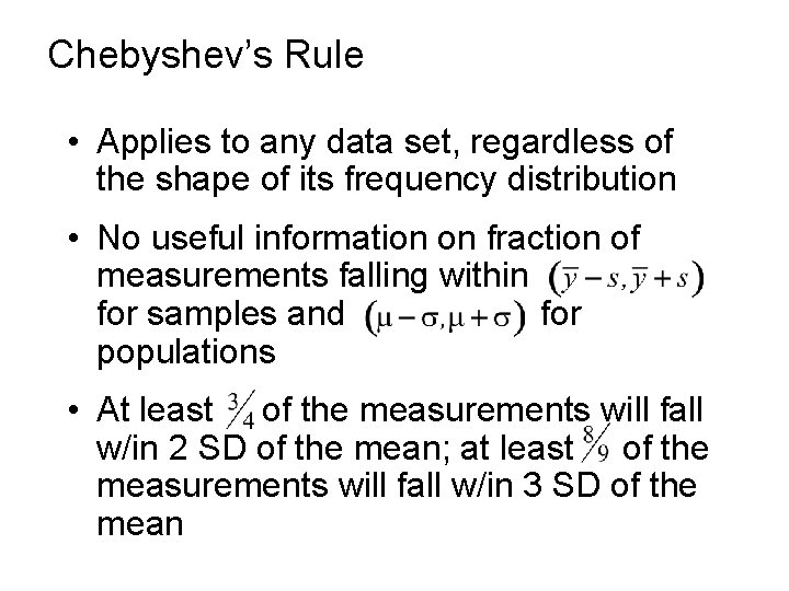
Chebyshev’s Rule • Applies to any data set, regardless of the shape of its frequency distribution • No useful information on fraction of measurements falling within for samples and for populations • At least of the measurements will fall w/in 2 SD of the mean; at least of the measurements will fall w/in 3 SD of the mean

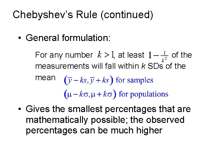
Chebyshev’s Rule (continued) • General formulation: For any number , at least of the measurements will fall within k SDs of the mean • Gives the smallest percentages that are mathematically possible; the observed percentages can be much higher

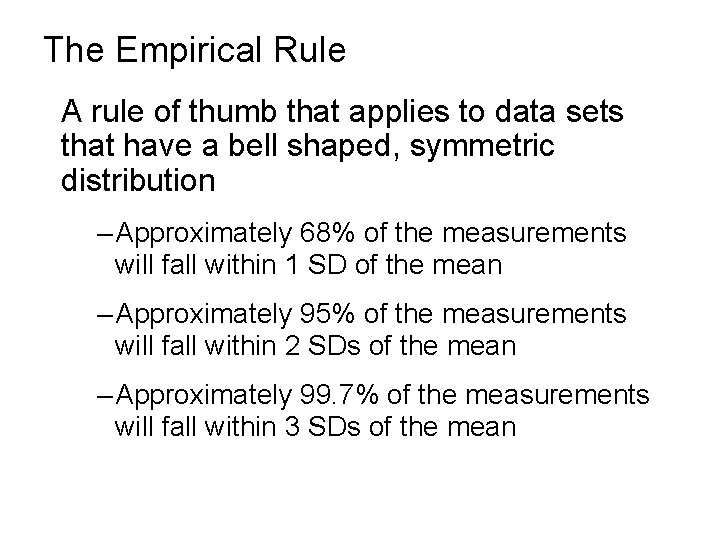
The Empirical Rule A rule of thumb that applies to data sets that have a bell shaped, symmetric distribution – Approximately 68% of the measurements will fall within 1 SD of the mean – Approximately 95% of the measurements will fall within 2 SDs of the mean – Approximately 99. 7% of the measurements will fall within 3 SDs of the mean

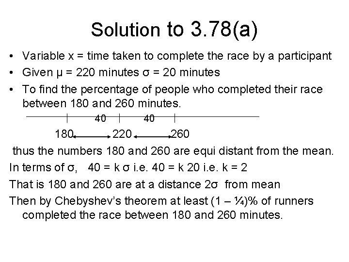
Solution to 3. 78(a) • Variable x = time taken to complete the race by a participant • Given µ = 220 minutes σ = 20 minutes • To find the percentage of people who completed their race between 180 and 260 minutes. 40 40 180 220 260 thus the numbers 180 and 260 are equi distant from the mean. In terms of σ, 40 = k σ i. e. 40 = k 20 i. e. k = 2 That is 180 and 260 are at a distance 2σ from mean Then by Chebyshev’s theorem at least (1 – ¼)% of runners completed the race between 180 and 260 minutes.

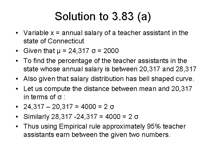
Solution to 3. 83 (a) • Variable x = annual salary of a teacher assistant in the state of Connecticut • Given that µ = 24, 317 σ = 2000 • To find the percentage of the teacher assistants in the state whose annual salary is between 20, 317 and 28, 317 • Also given that salary distribution has bell shaped curve. • Let us compute the distance between mean and 20, 317 in terms of σ : • 24, 317 – 20, 317 = 4000 = 2 σ • Similarly 28, 317 -24, 317 = 4000 = 2 σ • Thus using Empirical rule approximately 95% teacher assistants earn between the given two numbers.

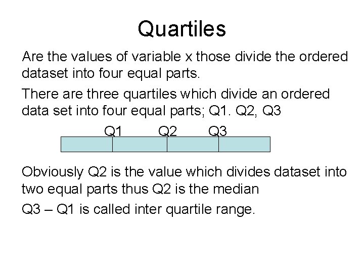
Quartiles Are the values of variable x those divide the ordered dataset into four equal parts. There are three quartiles which divide an ordered data set into four equal parts; Q 1. Q 2, Q 3 Q 1 Q 2 Q 3 Obviously Q 2 is the value which divides dataset into two equal parts thus Q 2 is the median Q 3 – Q 1 is called inter quartile range.

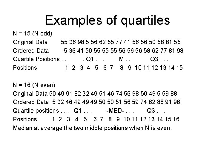
Examples of quartiles N = 15 (N odd) Original Data 55 36 98 5 56 62 55 77 41 56 56 50 58 81 55 Ordered Data 5 36 41 50 55 55 55 56 56 56 58 62 77 81 98 Quartile Positions. . . Q 1. . . M. . Q 3. . . Positions 1 2 3 4 5 6 7 8 9 10 11 12 13 14 15 N = 16 (N even) Original Data 50 49 91 82 32 49 51 46 74 56 98 50 49 5 59 88 Ordered Data 5 32 46 49 49 49 50 50 51 56 59 74 82 88 91 98 Quartile positions. . . Q 1. . . -MED-. . . Q 3. . . Positions 1 2 3 4 5 6 7 8 9 10 11 12 13 14 15 16 Median at average the two middle positions when N is even.

Box plots • To draw a box plot for the given dataset we need five summary measures • Max value, Min value and three quartiles • Inner fences = 1. 5 * inter quartile range • We will draw box plots with the help of minitab.