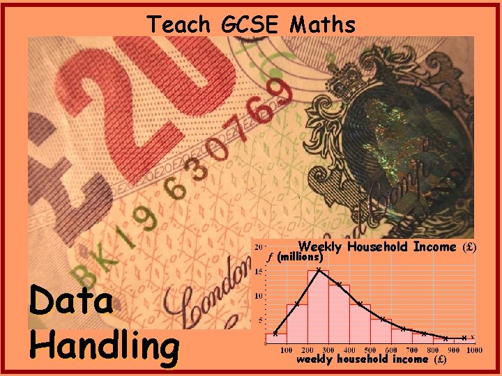
Teach GCSE Maths Weekly Household Income f millions

Teach GCSE Maths Weekly Household Income (£) f (millions) Data Handling x x x x x weekly household income (£) x

The pages that follow are sample slides from the 30 presentations that cover the work for Data Handling. A Microsoft WORD file, giving more information, is included in the folder. The animations pause after each piece of text. To continue, either click the left mouse button, press the space bar or press the forward arrow key on the keyboard. Animations will not work correctly unless Powerpoint 2002 or later is used.

F 1: The 3 Ms and Range The following extract comes from the 1 st foundation presentation. Here the students are shown the importance of ordering the data when finding the median.

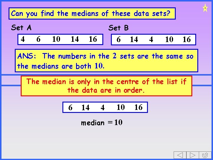
Can you find the medians of these data sets? Set A 4 Set B 6 10 14 16 6 14 4 10 16 ANS: The numbers in the 2 sets are the same so the medians are both 10. The median is only in the centre of the list if the data are in order. 6 14 4 10 median = 10 16

F 9: Reading Stem and Leaf Diagrams The work on stem and leaf diagrams gives an opportunity to revise the method of finding the median. This is shown on the next slide.

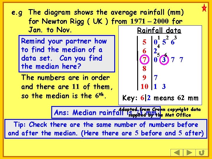
e. g The diagram shows the average rainfall (mm) for Newton Rigg ( UK ) from 1971 – 2000 for Jan. to Nov. Rainfall data Remind your partner how to find the median of a data set. Can you find the median here? The numbers are in order and there are 11 of them, so the median is the 6 th. 5 6 7 8 9 10 Key: 6 2 1 2 3 04 5 6 25 6 0 3 7 7 7 1 3 means 62 mm Adapted from Crown copyright data Ans: Median rainfall is 73 mm supplied by the Met Office Tip: Check there are the same number of numbers before and after the median. (Here there are 5 before and 5 after)

F 12: Histograms – Equal Class Widths A short summary is provided in each presentation in a form suitable for note-taking. The next slide shows the summary for the introductory work on histograms.

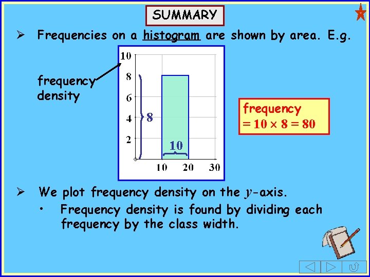
SUMMARY Ø Frequencies on a histogram are shown by area. E. g. frequency density frequency 8 = 10 8 = 80 10 Ø We plot frequency density on the y-axis. • Frequency density is found by dividing each frequency by the class width.

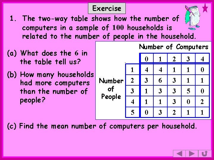
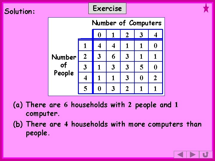
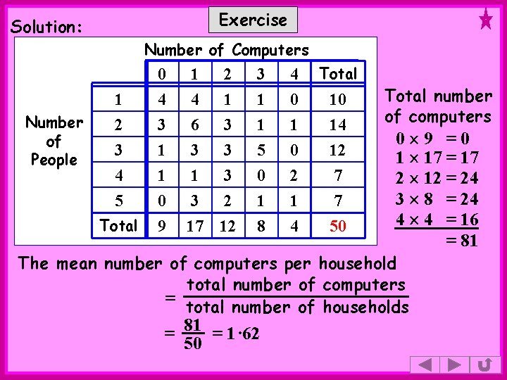
F 14: Two-Way Tables In addition to the questions asked of students as theory is being developed, there are short exercises to check that the main points have been understood. The icon in the top right hand corner indicates that in this exercise a calculator is not required.

Exercise 1. The two-way table shows how the number of computers in a sample of 100 households is related to the number of people in the household. (a) What does the 6 in the table tell us? (b) How many households had more computers Number of than the number of People people? Number of Computers 0 1 2 3 4 1 1 0 2 3 4 6 3 1 1 3 3 5 0 4 1 1 3 0 2 5 0 3 2 1 1 (c) Find the mean number of computers per household.

Exercise Solution: Number of Computers Number of People 1 2 3 0 4 3 1 1 4 6 3 2 1 3 3 3 1 1 5 4 0 1 0 4 5 1 0 1 3 3 2 0 1 2 1 (a) There are 6 households with 2 people and 1 computer. (b) There are 4 households with more computers than people.

Exercise Solution: Number of Computers Number of People 1 2 3 4 5 Total 0 4 3 1 1 4 6 3 2 1 3 3 3 1 1 5 4 0 1 0 Total 1 0 9 1 3 3 2 17 12 0 1 8 2 1 4 7 7 50 10 14 12 Total number of computers 0 9 =0 1 17 = 17 2 12 = 24 3 8 = 24 4 4 = 16 = 81 The mean number of computers per household total number of computers = total number of households = 81 = 1· 62 50

H 3: Box Plots As well as showing students how to draw box plots, the presentation on box plots uses real data to illustrate the usefulness of the diagrams when comparing data.

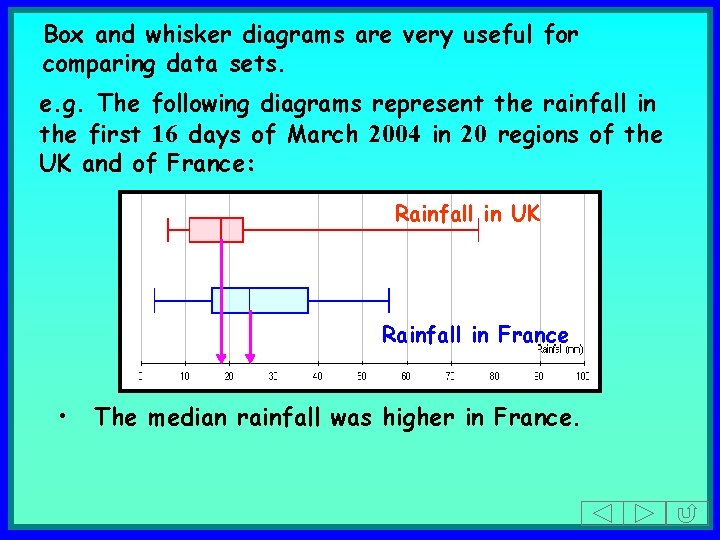
Box and whisker diagrams are very useful for comparing data sets. e. g. The following diagrams represent the rainfall in the first 16 days of March 2004 in 20 regions of the UK and of France: Rainfall in UK Rainfall in France • The median rainfall was higher in France.

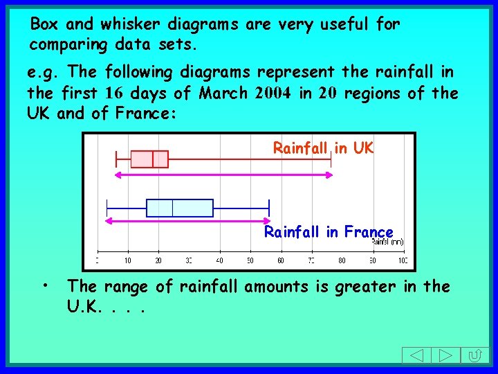
Box and whisker diagrams are very useful for comparing data sets. e. g. The following diagrams represent the rainfall in the first 16 days of March 2004 in 20 regions of the UK and of France: Rainfall in UK Rainfall in France • The range of rainfall amounts is greater in the U. K. .

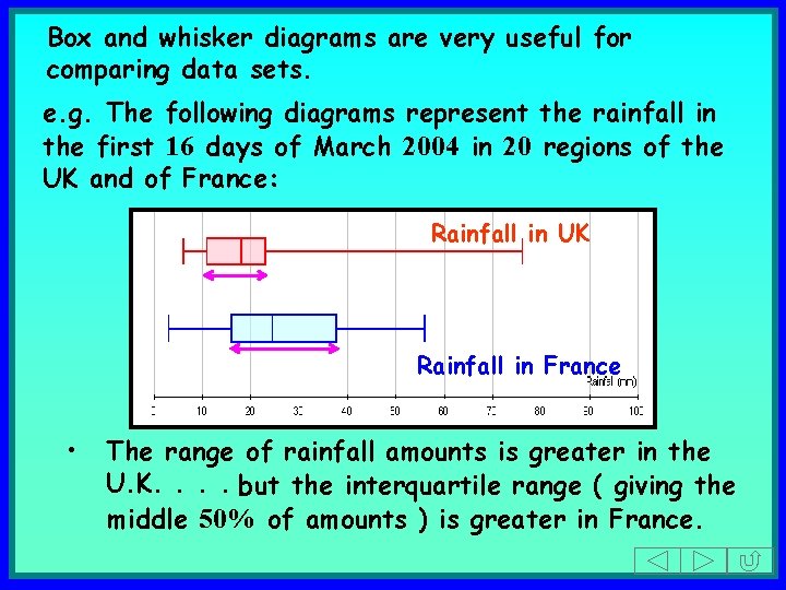
Box and whisker diagrams are very useful for comparing data sets. e. g. The following diagrams represent the rainfall in the first 16 days of March 2004 in 20 regions of the UK and of France: Rainfall in UK Rainfall in France • The range of rainfall amounts is greater in the U. K. . but the interquartile range ( giving the middle 50% of amounts ) is greater in France.

H 6: Probability and Independent Events It is important for students to recognise the difference between independent events and those that are not independent. The presentation gives examples of situations involving both types.

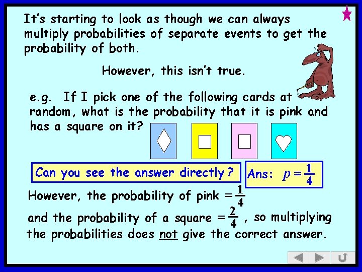
It’s starting to look as though we can always multiply probabilities of separate events to get the probability of both. However, this isn’t true. e. g. If I pick one of the following cards at random, what is the probability that it is pink and has a square on it? Ans: p = 1 Can you see the answer directly ? However, the probability of pink = 1 4 4 2 , so multiplying and the probability of a square = 4 the probabilities does not give the correct answer.

The next 2 slides contain a list of the 30 files that make up Data Handling. The files have been labelled as follows: F: Topics for the Foundation level. H: Topics which appear only in the Higher level content. Also for ease of access, colours have been used to group topics. For example, blue is used at both levels for work on probability. The 2 underlined titles contain links to the complete files that are included in this sample.

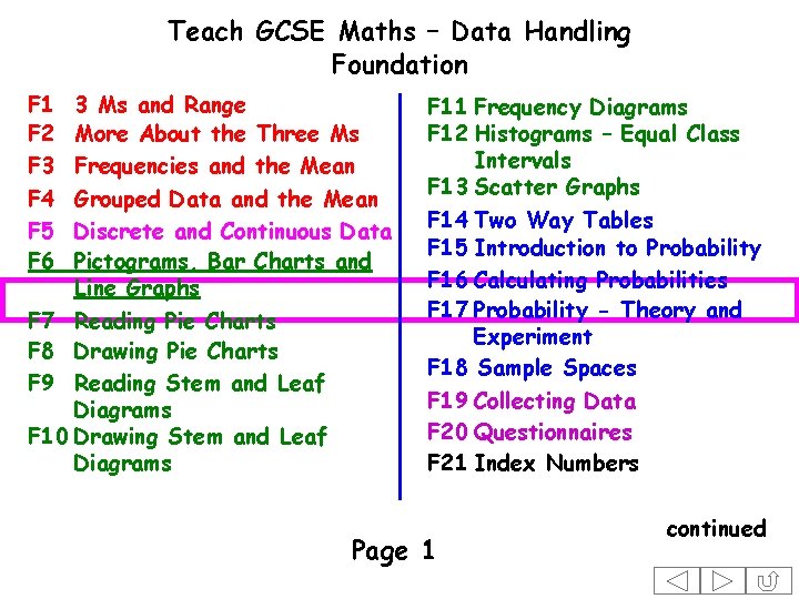
Teach GCSE Maths – Data Handling Foundation F 1 F 2 F 3 F 4 F 5 F 6 3 Ms and Range More About the Three Ms Frequencies and the Mean Grouped Data and the Mean Discrete and Continuous Data Pictograms, Bar Charts and Line Graphs F 7 Reading Pie Charts F 8 Drawing Pie Charts F 9 Reading Stem and Leaf Diagrams F 10 Drawing Stem and Leaf Diagrams F 11 Frequency Diagrams F 12 Histograms – Equal Class Intervals F 13 Scatter Graphs F 14 Two Way Tables F 15 Introduction to Probability F 16 Calculating Probabilities F 17 Probability - Theory and Experiment F 18 Sample Spaces F 19 Collecting Data F 20 Questionnaires F 21 Index Numbers Page 1 continued

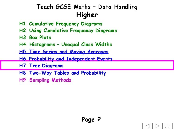
Teach GCSE Maths – Data Handling Higher H 1 H 2 H 3 H 4 H 5 H 6 H 7 H 8 H 9 Cumulative Frequency Diagrams Using Cumulative Frequency Diagrams Box Plots Histograms – Unequal Class Widths Time Series and Moving Averages Probability and Independent Events Tree Diagrams Two-Way Tables and Probability Sampling Methods Page 2