Survey of program slicing techniques Presenters Name Keyur

Survey of program slicing techniques Presenter’s Name: Keyur Malaviya

Purpose of this paper ¢ ¢ ¢ It’s a survey that presents an overview of program slicing Various general approaches used to compute slices Specific techniques used to address procedures, unstructured control flow, composite data types and pointers, and concurrency. Static and dynamic slicing methods for each of these features Comparison and classification in terms of their accuracy and efficiency

Topics Covered ¢ ¢ Definitions Static slicing vs Dynamic slicing Basic slicing algorithm for single procedure and multiprocedure l Weiser Algorithm l Hausler l Bergeretti and Carr´e l Horwitz, Reps, and Binkley Algo Applications

Definitions (Basics) ¢ ¢ ¢ (1) read(n); (2) i : = 1; Slicing? (3) sum : = 0; Slicing (4) product. Criteria? : = 1; (5) while i <= n do Static and Dynamic slicing? begin (6) sum : = sum + i; Program slicing? (7) product : = product * i; Program (8) i : = i + 1 dependence graph (PDG) end; Control flow graph (CFG) or (9) write(sum); (10) write(product) System dependency grapy (SDG) or

Definitions (CFG PDG) PDG: Directed graph; Vertices = CFG statements and control predicates Edges = data and control dependences

Definitions ¢ Program slice: consists of the parts of a program that affect the values computed at some point of interest. ¢ Slicing criterion: is this point of interest specified by a pair (program point, set of variables) ¢ Original concept by Weiser: Its a mental abstractions that people make when they are debugging a program ¢ Static slicing: Computed without making assumptions regarding a program’s input ¢ Dynamic slicing: Relies on some specific test case

Definitions (criteria and slicing ) Slice of this program w. r. t criterion (10, product) (1) read(n); (2) i : = 1; (3) sum : = 0; (4) product : = 1; (5) while i <= n do begin (6) sum : = sum + i; (7) product : = product * i; (8) i : = i + 1 end; (9) write(sum); (10) write(product) (1) read(n); (2) i(2) : = i 1; : = 1; (3) sum (3) : = 0; (4) product : = 1; (5) while i <=i n<=do n do begin (6) sum (6) : = sum + i; (7) product : = product * i; (8) i(8) : = ii : = + 1 i + 1 end; (9) write(sum); (9) (10) write(product) Single-procedure programs (PDG); Shading in the PDG shown before vertices in the slice w. r. t.

Static slicing vs Dynamic slicing ¢ Dynamic Slicing: First introduced by Korel and Laski Non-interactive variation of Balzer’s flowback analysis Flowback Only the dependences analysis: Interactively that occurtraverse in a specific a graph execution (data and of the program are taken into account control dependences between statements in the program); For S(V) depends on T(V), is S and T are statements; T of. Sais ¢ e. g. : Dynamic slicing criterion a triple (input, occurrence – it from specifies the and distinguishes instatement, CFG, thenvariable) trace back vertex forinput, S to vertex for T between different occurrences of a statement in the execution history ¢ Dynamic slicing assumes fixed input for a program ¢ Static slicing does not make assumptions regarding the input. ¢

Static slicing vs Dynamic slicing criterion SS: (8, x) and DS: (n=2, 81, x) Example program: Static slice w. r. t. criterion (8, x) Dynamic slice w. r. t. criterion (n=2, 81, x) 1 read(n); 2 i : = 1; 3 while (i <= n) do begin 4 if (i mod 2 = 0) then 5 x : = 17 else 6 x : = 18; 7 i : = i + 1 end; 8 write(x) read(n); i : = 1; while (i <= n) do begin if (i mod 2 = 0) then x : = 17 else x : = 18; i : = i + 1 end; write(x) read(n); i : = 1; while (i <= n) do begin if (i mod 2 = 0) then x : = 17 else ; i : = i + 1 end; write(x)

Slicing Algorithm Approaches ¢ Achieved through one of three algorithmic approaches: 1) data-flow equations 2) system dependency graph 3) parallel algorithm ¢ All based on control and data dependencies and defined in terms of a graph representation of a program (as seen before)

Approaches: ¢ ¢ Weiser’s approach: slices from Statements and controlcompute predicates are gathered by consecutive sets oftraversal transitively relevant way of a backward of the program’s statements ( data flow and control flow graph dependences ) (CFG) or PDG, starting at the slicing criterion ¢ ¢ Ottenstein approach: in terms of a reachability problem in a PDG. Slicing criterion A vertex in the PDG; A Slice corresponds to all PDG vertices from which the vertex under consideration can be reached Other approaches: Based on modified and extended versions of PDGs

Weiser Algorithm (single procedure) ¢ Two levels of iteration: 1. Transitive data dependences in the presence of loops in the program 2. Control dependences, initiating the inclusion of control predicates for which each, step 1 is repeated to include the statements it is dependent upon ¢ Determine directly relevant variables and then indirectly relevant variables; From these compute the sets of relevant statements

Parameters and equations ¢ Defined and Referenced Variables DEF(i) and REF(i) l Say at node ‘i’ consider a statement a=b+c l Then DEF(i) = {a} and REF(i) = {b, c} l ¢ Directly Relevant Variable l l : set of directly relevant variables, where slice criterion = (V, n) Set DRV (i) Set DRV (all nodes j) that have a direct edge to i,

Parameters and equations ¢ Directly Relevant Statements l ¢ : set of all nodes i that define a variable v that is relevant at the successor node of I Indirectly Relevant Variables l referenced variables in control predicate are indirectly relevant when at least one of the statements in its body is relevant, denoted: l b is known as a range of influence INFL (b),

Example program

Applying the Weiser algo Slicing criterion (10, product) & our example program NODE DEF REF 1 {n} 0 0 2 {i} 0 0 3 {sum} 0 0 4 {product} 0 0 5 0 {i, n} {6, 7, 8} 6 {sum} {sum, i} 0 7 {product} {product, i} 0 8 {i} 0 9 0 {sum} 0 10 0 {product} INFLR 0 {product} 0

Applying the Weiser algo Slicing criterion (10, product) & our example program NODE DEF REF 1 {n} 0 2 {i} 0 3 {sum} 0 4 {product} 0 5 0 {i, n} 6 {sum} {sum, i} 7 {product} {product, i} 8 {i} {product} 9 0 {sum} 10 0 {product} R 0

Applying the Weiser algo Slicing criterion (10, product) & our example program NODE DEF REF 1 {n} 0 2 {i} 0 3 {sum} 0 4 {product} 0 5 0 {i, n} 6 {sum} {sum, i} 7 {product} {product, i} 8 {i} {product} 9 0 {sum} 10 0 {product} R 0

Applying the Weiser algo (10, {i, product) & ourthe example program Slicing criterion (5, n}) & repeat same procedure NODE DEF REF 1 {n} 0 R 0 0 2 {i} 0 0 0 {n} 3 {sum} 0 {i} {i, n} 4 {product} 0 {i} {i, n} 5 0 {i, n} {product, i, n} 6 {sum} {sum, i} {product, i} 7 {product} {product, i} 8 {i} {product, i} 9 0 {sum} {product} 10 0 {product} {product, i, n} {product}

Applying the Weiser algo Slicing criterion (10, product) & our example program NODE DEF REF INFL R 0 R 1 1 {n} 0 0 2 {i} 0 0 0 {n} 3 {sum} 0 0 {i} {i, n} 4 {product} 0 0 {i} {i, n} 5 0 {i, n} {6, 7, 8} {product, i, n} 6 {sum} {sum, i} 0 {product, i} {product, i, n} 7 {product} {product, i} 0 {product, i} {product, i, n} 8 {i} 0 {product, i} {product, i, n} 9 0 {sum} 0 {product} 10 0 {product} ? ? ?

Equations for related statements:

Hausler (functional style) ¢ ¢ ¢ For each type of statement, have a function and & express how a statement transforms the set of relevant variables & relevant statements reply. Functions for a while statement are obtained by transforming it into an infinite sequence of if statements

Information-flow relations (Bergeretti and Carr´e) Statement S: variable v and an expression e ( e can be control predicate or right-hand side of assignment) ¢ We define relations: ¢ They possess following properties: iff the value of v on entry to S potentially affects the value computed for e iff the value computed for e potentially affects the value of v on exit from S, iff the value of v on entry to S may affect the value of v on exit from S.

Information-flow relations (Bergeretti and Carr´e) ¢ How to get the slice with respect to the final value of v ? The set of all expressions e for which can be used to construct “partial statements” replace all statements in S that do not contain expressions in by empty statements. Relations are computed in a syntax-directed, bottom-up ¢ For S, v : = e ¢ ¢

Information-flow relations (Bergeretti and Carr´e) ¢ Set of expressions that potentially affect the value of product at the end of the program are {1, 2, 4, 5, 7, 8} ¢ Partial statement is obtained by omitting all statements from the program that do not contain expressions in this set, i. e. , both assignments to sum and both write statements ¢ The slice is same as Weiser’s algorithm

Dependence graph based approaches (PDG) and Procedures ¢ ¢ ¢ PDG variant of Ottenstein shows considerably more detail than that by Horwitz, Reps, and Binkley Procedures l Call-return structure of interprocedural execution paths l Single pass considers infeasible execution paths – a problem called “calling-context” Will see two approaches: l Weiser’s approach (CFG) l Horwitz, Reps, and Binkley (SDG)

Dependence graph based approaches (PDG) and Procedures ¢ Weiser’s approach for interprocedural static slicing: l Interprocedural summary information is computed, using previously developed techniques P, set MOD(P) of variables = modified by P, and l set USE(P) of variables = used by P Intraprocedural slicing algorithm: Treat ‘P()’ as a conditional assignment statement ‘if Some. Predicate then MOD(P) : = USE(P)’ (external procedures, source-code is unavailable? )

Weiser’s approach ¢ Actual inter-procedural slicing algo that generates new slicing criteria iteratively w. r. t slices computed in step (2): l (i) Q called by P: consist of all (i) procedures Q called pairs (ii) procedures R that call P l (ii) procedures R that call P: consist of all l l pairs

Weiser’s Algo ¢ ¢ ¢ To formalize the generation of new criteria: UP(S) : Map (a set S of slicing criteria in a P) to (a set of criteria in procedures that call P) DOWN(S): Map (a set S of slicing criteria in a P) to (a set of criteria in procedures called by P) Set of all criteria: transitive and reflexive closure of the UP and DOWN relations (UP U DOWN)* UP and DOWN sets: Requires sets of relevant variables to be known at all call sites computation of these sets is done by slicing these procedures When iteration stops? l When no new criteria are generated

Main issue: ¢ ¢ ¢ ¢ program Main; … while ( ) do P(x 1, x 2, , xn); z : = x 1; x 1 : = x 2; x 2 : = x 3; procedure P(y 1, y 2, … , yn); begin write(y 1); write(y 2); … (M) write(yn) end ¢ ¢ ¢ xn 1 : = xn end; (L) write(z) end Procedure P is sliced ‘n’ times by Weiser’s algorithm for criterion (L, {z}).

Weiser’s Algo ¢ ¢ ¢ L program point at S = write(z) M program point at last statement in P Slice w. r. t. criterion (L, { z })? l ‘n’ iterations of the body of the while loop l During the ith iteration, variables x 1, …, xi will be relevant at call site l DOWN(Main): criterion (M, { y 1, …, yi }) gets included Procedure P will be sliced n times l Issue is: ? ? ?

What was the problem? ¢ Weiser’s algorithm does not take into account which output parameters are dependent on which input parameters is a source of imprecision ¢ Lets see another examples that shows this problem:

What was the problem? program Example; begin (1) a : = 17; (2) b : = 18; (3) P(a, b, c, d); (4) write(d) end procedure P(v, w, x, y); (5) x : = v; (6) y : = w end program Example; begin ; a : =17; b : = 18; : =c, 18; P(a, b b, d); write(d) P(a, b, c, d); end procedure P(v, w, x, y); ; procedure P(v, w, x, y); y : =; w endy : = w end Slice with Actual Slice Weiser’s algo

Horwitz, Reps, and Binkley Algo ¢ Computes precise inter-procedural static slices: ¢ 1. SDG, a graph representation for multi-procedure programs 2. Computation of inter-procedural summary information l precise dependence relations between i/p & o/t parameters l explicitly present in SDG as summary edges 3. Two-pass algorithm for extracting interprocedural slices from an SDG ¢ ¢

Multi-procedure program

Horwitz, Reps, and Binkley Algo 1) Structure of SDG ¢ ¢ ¢ SDG = PDG for main program, & a procedure dependence graph for each procedure SDG <> PDG (Vertices and edges are different) For each call statement, there is a call-site vertex in the SDG as well as actual-in and actual-out vertices

1) Structure of SDG Each procedure dependence graph has an entry vertex, and formal-in and formal-out vertices ¢ ¢ interprocedural dependence edges: (i) control dependence edge (call-site vertex & entry vertex) (ii) parameter-in edge between corresponding actual-in and formal-in vertices, (iii) a parameter out edge between corresponding formal-out and actual-out vertices, and (iv) summary edges that represent transitive interprocedural data dependences

1) Structure of SDG

Horwitz, Reps, and Binkley Algo 2) and 3) ¢ Second part: l Models the calling relationships between the procedures (as in a call graph) Compute subordinate characteristic graph For each procedure in the program, this graph contains edges that correspond to precise transitive flow dependences between its input and output parameters. l l ¢ l l l Third part: summary edges of an SDG serve to circumvent the calling context problem First phase: all vertices from which ‘s’ can be reached without descending into procedure calls (slicing starts at vertex s) Second phase: remaining vertices in the slice by descending into all previously side-stepped calls

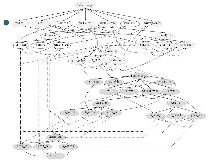
COMPLETE SDG NEXT: Complete SDG for the example program shown above

SDG style interpretation ¢ ¢ ¢ ¢ Thin solid arrows represent flow dependences, Thick solid arrows correspond to control dependences, Thin dashed arrows Used for call, parameter-in, and parameter-out dependences, Thick dashed arrows Transitive inter-procedural flow dependences. Shaded vertices Vertices in the slice w. r. t. statement write(product) Light shading Vertices identified in the first phase Dark shading Vertices identified in the second phase

The slice with criteria (10, product) program Example; begin (1) read(n); (2) i : = 1; (3) sum : = 0; (4) product : = 1; (5) while i <= n do begin (6) Add(sum, i); (7) Multiply(product, i); (8) Add(i, 1) end; (9) write(sum); (10) write(product) end procedure Add(a; b); begin 11) a : = a + b End procedure Multiply(c; d); begin 12) j : = 1; 13) k : = 0; 14) while j <= d do begin 15) Add(k, c); 16) Add(j, 1); end; 17) c : = k end

Application of slicing ¢ ¢ Debugging and program analysis Program differencing and program integration l l l ¢ analyzing an old and a new version of a program partitioning the components compares slices in order to detect equivalent behaviors Software maintenance l change at some place in a program behavior of other parts of the program

¢ QUESTIONS