Suffix tree and suffix array techniques for pattern

Suffix tree and suffix array techniques for pattern analysis in strings Esko Ukkonen Univ Helsinki Erice School 30 Oct 2005 Modified Alon Itai 2006 1

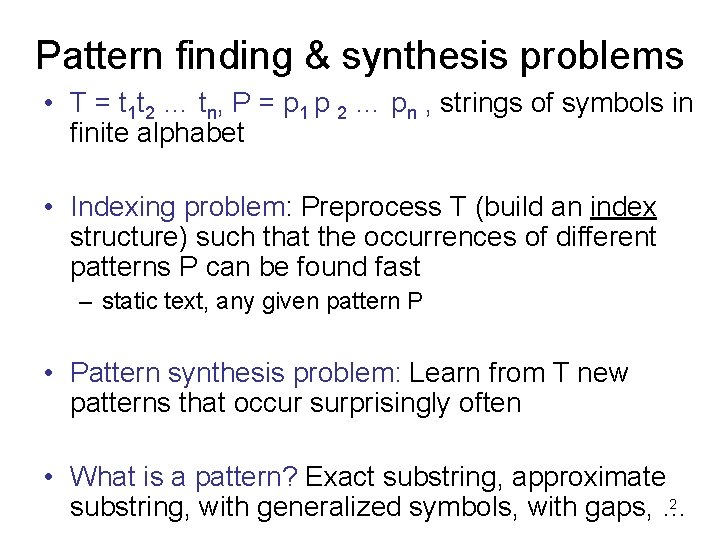
Pattern finding & synthesis problems • T = t 1 t 2 … tn, P = p 1 p 2 … pn , strings of symbols in finite alphabet • Indexing problem: Preprocess T (build an index structure) such that the occurrences of different patterns P can be found fast – static text, any given pattern P • Pattern synthesis problem: Learn from T new patterns that occur surprisingly often • What is a pattern? Exact substring, approximate 2 substring, with generalized symbols, with gaps, …

1. Suffix tree 2. Suffix array 3. Some applications 4. Finding motifs 3

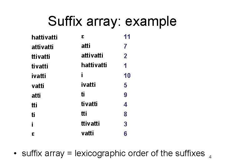
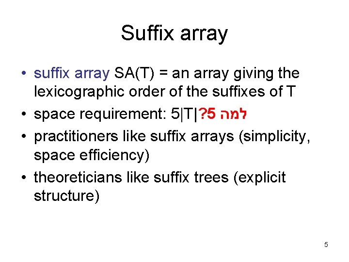
Suffix array: example hattivatti ε 11 attivatti 7 ttivattivatti 2 tivatti hattivatti 1 ivatti i 10 vatti ivatti 5 atti ti 9 tti tivatti 4 ti tti 8 i ttivatti 3 ε vatti 6 • suffix array = lexicographic order of the suffixes 4

Suffix array • suffix array SA(T) = an array giving the lexicographic order of the suffixes of T • space requirement: 5|T|? 5 למה • practitioners like suffix arrays (simplicity, space efficiency) • theoreticians like suffix trees (explicit structure) 5

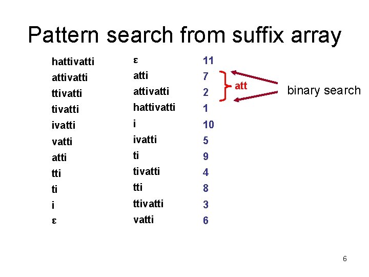
Pattern search from suffix array hattivatti ε 11 attivatti 7 ttivattivatti 2 tivatti hattivatti 1 ivatti i 10 vatti ivatti 5 atti ti 9 tti tivatti 4 ti tti 8 i ttivatti 3 ε vatti 6 att binary search 6

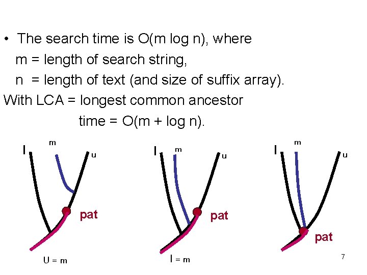
• The search time is O(m log n), where m = length of search string, n = length of text (and size of suffix array). With LCA = longest common ancestor time = O(m + log n). l m u l m pat u l m u pat U=m l=m 7

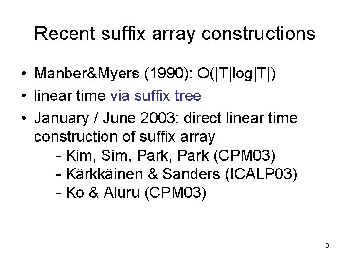
Recent suffix array constructions • Manber&Myers (1990): O(|T|log|T|) • linear time via suffix tree • January / June 2003: direct linear time construction of suffix array - Kim, Sim, Park (CPM 03) - Kärkkäinen & Sanders (ICALP 03) - Ko & Aluru (CPM 03) 8

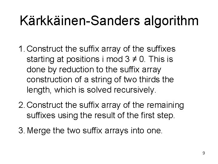
Kärkkäinen-Sanders algorithm 1. Construct the suffix array of the suffixes starting at positions i mod 3 ≠ 0. This is done by reduction to the suffix array construction of a string of two thirds the length, which is solved recursively. 2. Construct the suffix array of the remaining suffixes using the result of the first step. 3. Merge the two suffix arrays into one. 9

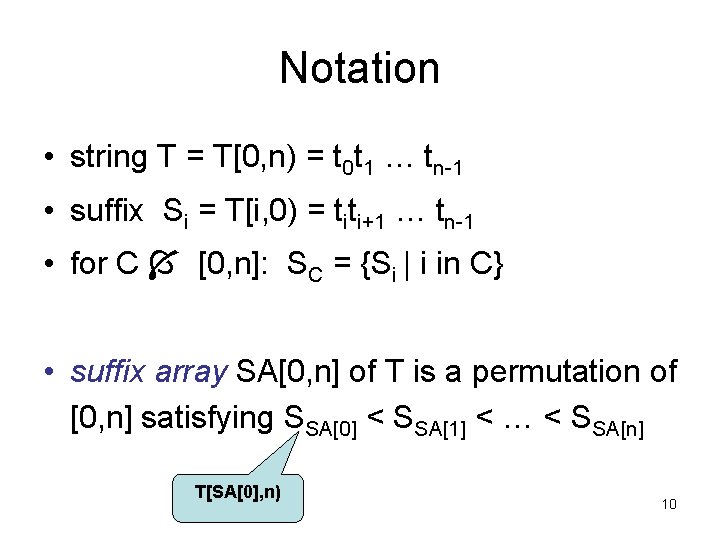
Notation • string T = T[0, n) = t 0 t 1 … tn-1 • suffix Si = T[i, 0) = titi+1 … tn-1 • for C [0, n]: SC = {Si | i in C} • suffix array SA[0, n] of T is a permutation of [0, n] satisfying SSA[0] < SSA[1] < … < SSA[n] T[SA[0], n) 10

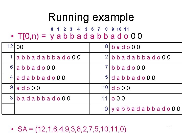
Running example 0 1 2 3 4 5 6 7 8 9 10 11 • T[0, n) = y a b b a d o 0 0 12 00 8 bado 00 1 abbado 00 2 bbadabbado 00 6 abbado 00 7 bbado 00 4 adabbado 00 5 dabbado 00 9 ado 00 10 3 badabbado 00 11 o 0 0 do 00 0 yabbado 00 • SA = (12, 1, 6, 4, 9, 3, 8, 2, 7, 5, 10, 11, 0) 11

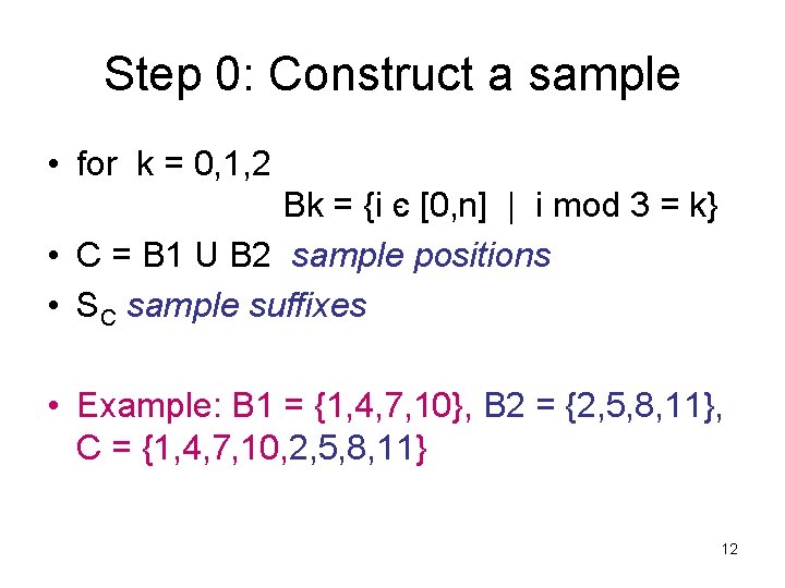
Step 0: Construct a sample • for k = 0, 1, 2 Bk = {i є [0, n] | i mod 3 = k} • C = B 1 U B 2 sample positions • SC sample suffixes • Example: B 1 = {1, 4, 7, 10}, B 2 = {2, 5, 8, 11}, C = {1, 4, 7, 10, 2, 5, 8, 11} 12

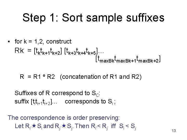
Step 1: Sort sample suffixes • for k = 1, 2, construct Rk = [tktk+1 tk+2] [tk+3 tk+4 tk+5]… [tmax. Bk+1 tmax. Bk+2] R = R 1 º R 2 (concatenation of R 1 and R 2) Suffixes of R correspond to SC: suffix [titi+1 ti+2]… corresponds to Si ; The correspondence is order preserving: Let Ri’ Si and Rj’ Sj. Then Ri’< Rj’ iff Si < Sj 13

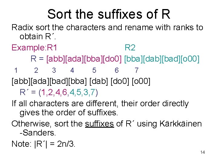
Sort the suffixes of R Radix sort the characters and rename with ranks to obtain R´. Example: R 1 R 2 R = [abb][ada][bba][do 0] [bba][dab][bad][o 00] 1 2 3 4 5 6 7 [abb][ada][bad][bba] [dab] [do 0] [o 00] R´ = (1, 2, 4, 6, 4, 5, 3, 7) If all characters are different, their order directly gives the order of suffixes. Otherwise, sort the suffixes of R´ using Kärkkäinen -Sanders. Note: |R´| = 2 n/3. 14

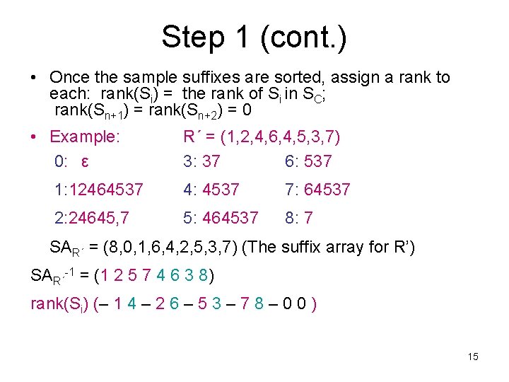
Step 1 (cont. ) • Once the sample suffixes are sorted, assign a rank to each: rank(Si) = the rank of Si in SC; rank(Sn+1) = rank(Sn+2) = 0 • Example: 0: ε R´ = (1, 2, 4, 6, 4, 5, 3, 7) 3: 37 6: 537 1: 12464537 4: 4537 7: 64537 2: 24645, 7 5: 464537 8: 7 SAR´ = (8, 0, 1, 6, 4, 2, 5, 3, 7) (The suffix array for R’) SAR´-1 = (1 2 5 7 4 6 3 8) rank(Si) (– 1 4 – 2 6 – 5 3 – 7 8 – 0 0 ) 15

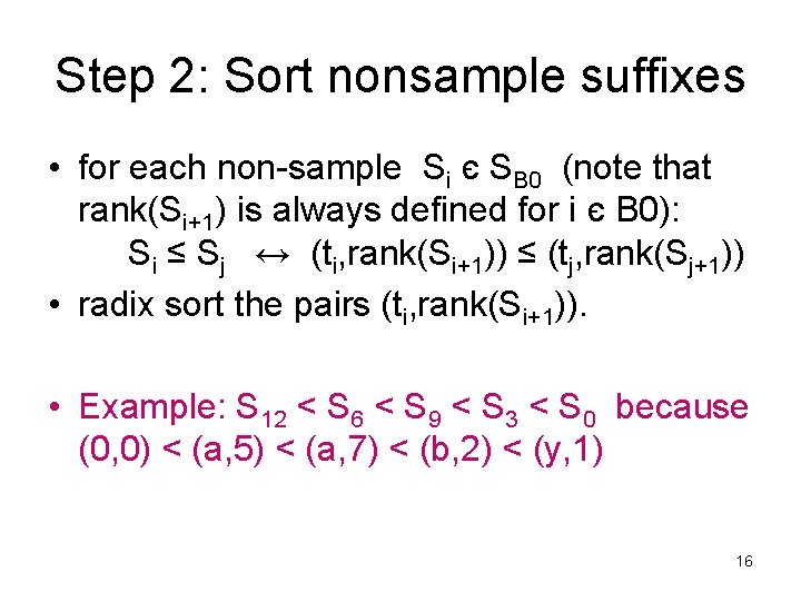
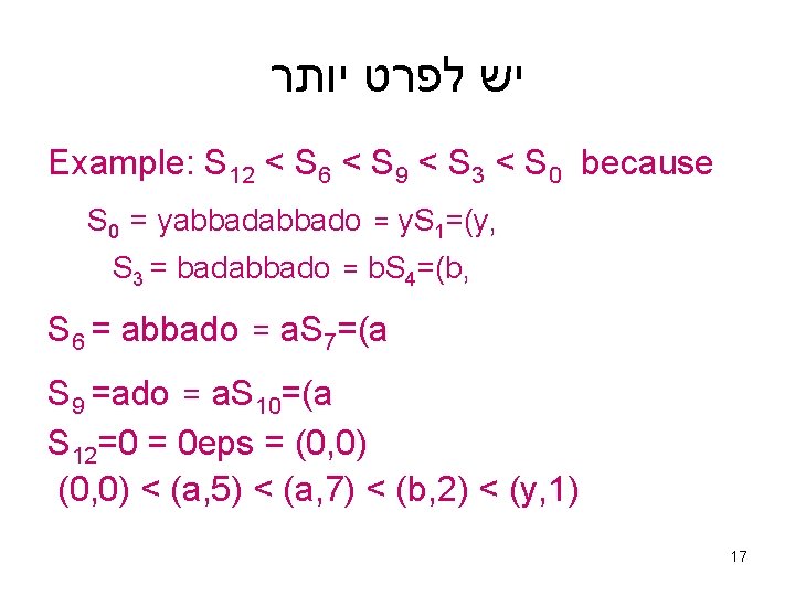
Step 2: Sort nonsample suffixes • for each non-sample Si є SB 0 (note that rank(Si+1) is always defined for i є B 0): Si ≤ Sj ↔ (ti, rank(Si+1)) ≤ (tj, rank(Sj+1)) • radix sort the pairs (ti, rank(Si+1)). • Example: S 12 < S 6 < S 9 < S 3 < S 0 because (0, 0) < (a, 5) < (a, 7) < (b, 2) < (y, 1) 16

יש לפרט יותר Example: S 12 < S 6 < S 9 < S 3 < S 0 because S 0 = yabbado = y. S 1=(y, S 3 = badabbado = b. S 4=(b, S 6 = abbado = a. S 7=(a S 9 =ado = a. S 10=(a S 12=0 = 0 eps = (0, 0) < (a, 5) < (a, 7) < (b, 2) < (y, 1) 17

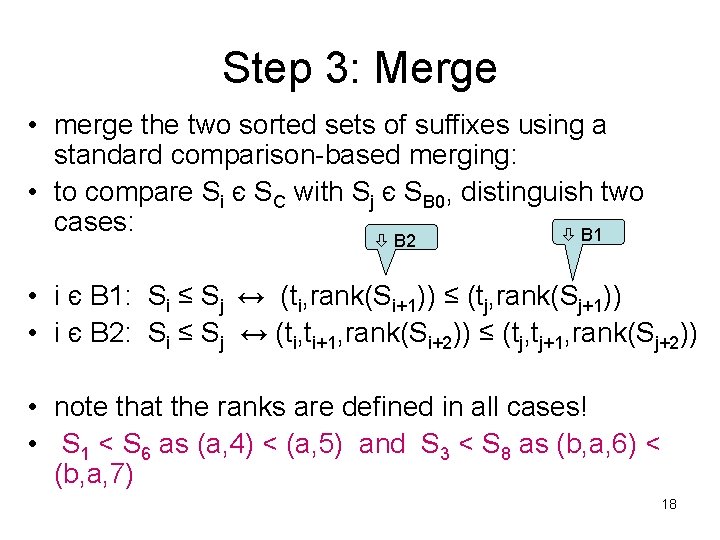
Step 3: Merge • merge the two sorted sets of suffixes using a standard comparison-based merging: • to compare Si є SC with Sj є SB 0, distinguish two cases: B 1 B 2 • i є B 1: Si ≤ Sj ↔ (ti, rank(Si+1)) ≤ (tj, rank(Sj+1)) • i є B 2: Si ≤ Sj ↔ (ti, ti+1, rank(Si+2)) ≤ (tj, tj+1, rank(Sj+2)) • note that the ranks are defined in all cases! • S 1 < S 6 as (a, 4) < (a, 5) and S 3 < S 8 as (b, a, 6) < (b, a, 7) 18

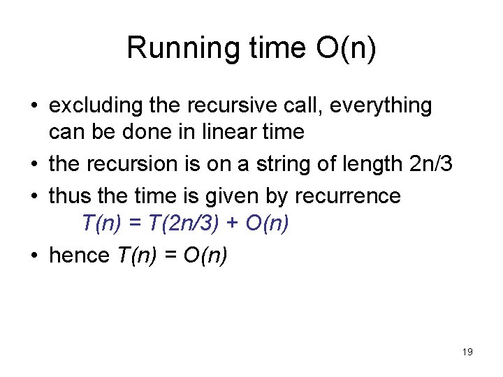
Running time O(n) • excluding the recursive call, everything can be done in linear time • the recursion is on a string of length 2 n/3 • thus the time is given by recurrence T(n) = T(2 n/3) + O(n) • hence T(n) = O(n) 19

Implementation • about 50 lines of C++ • code available e. g. via Juha Kärkkäinen’s home page 20

LCP table • Longest Common Prefix of successive elements of suffix array: • LCP[i] = length of the longest common prefix of suffixes SSA[i] and SSA[i+1] • Algorithm: • Enter the suffixes in a trie • Find the lca. • Complexity = O(n 2) 21

Kasai et al, CPM 2001 Key observation: Let LCP[q]=h>1, i. e. , S SA[q] = titi+1…ai+h-1 ti+h S SA[q+1]= tktk+1…tk+h-1 tk+h = titi+1…ti+h-1 ti+h ( tk+h≠ti+h) • Then ti+1…ti+h-1=tk+1…tk+h-1, . • Define p therefore SSA[p] =ti+1…ti+h-1… SSA[p+1]=ti+1…ti+h-1 … • i. e. , LCP[p] ≥ h-1 • When computing LCP[p] we can start the comparisons at position p+h-1. 22

The algorithm for(i=0; i<n; i++) /* compute SA-1 */ SA-1[SA[i]] = i; h = 0; for(p=0; p<n; p++) { if(SA-1[p] > 0){ r = SA [SA-1 [p]+1] ; innermost statement while(T[r+h] = T[p+h]) h++; LCP[SA-1 [p]] = h; Complexity: if(h > 0) Since h is decreased at most n times, h--; } and h ≤ n, } h can be increased at most 2 n times; i. e. , the innermost statement is executed ≤ 2 n times. Total time = O(n). 23

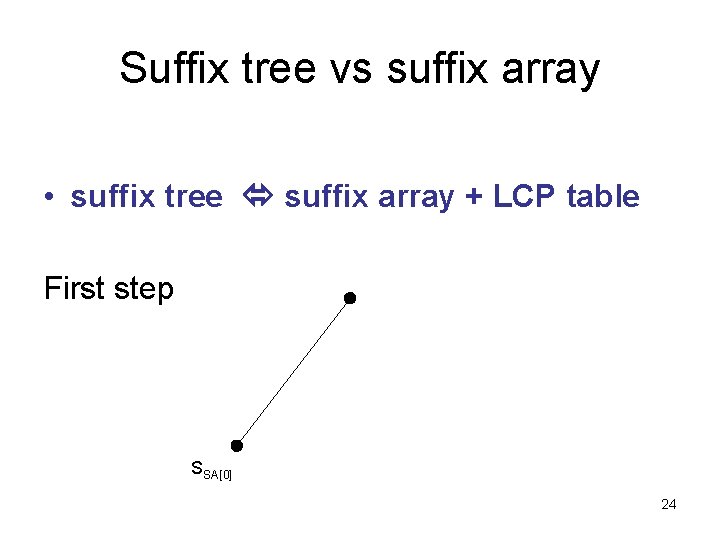
Suffix tree vs suffix array • suffix tree suffix array + LCP table First step SSA[0] 24

• Step i Which edge to split? SSA[0] S SA[i] SSA[i-1] Complexity: The final trie has 2 n vertices. Each edge is traversed ≤ twice. Time = O(n). 25