Algorithms in the Real World Suffix Trees Page

Algorithms in the Real World Suffix Trees Page 1

Exact String Matching • Given a text S of length m and pattern P of length n, “quickly” find an occurrence (or all occurrences) of P in S • A Naïve solution: Compare P with S[i…i+n-1] for all i --- O(nm) time • How about O(n+m) time? (Knuth-Morris-Pratt) – O(n) time to build a finite-state machine recognizing P (clever algorithm) – O(m) time to run S through finite-state machine • How about O(m) preprocessing time and O(n) search time? Page 2

Suffix Trees • Preprocess the text in O(m) time and search in O(n) time • Idea: – Construct a tree containing all suffixes of text along the paths from the root to the leaves – For search, just follow the appropriate path: if the pattern occurs in the text, then it is a prefix of some suffix of the text. Page 3

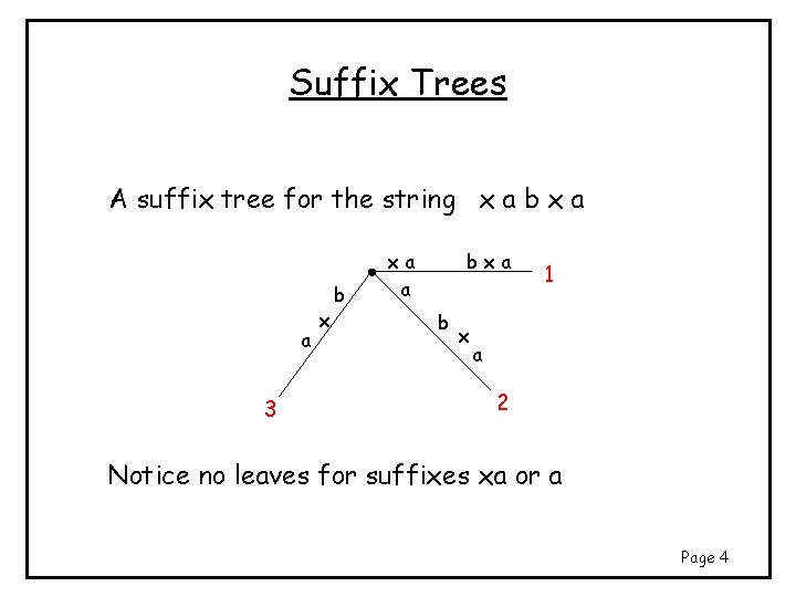
Suffix Trees A suffix tree for the string x a b x a a 3 x b xa a bxa b x 1 a 2 Notice no leaves for suffixes xa or a Page 4

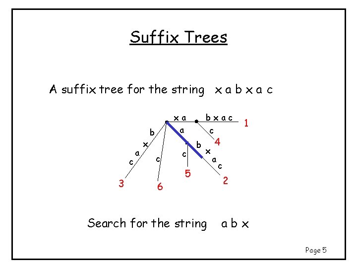
Suffix Trees A suffix tree for the string x a b x a c c 3 a x xa a b c 6 c bxac c b x 5 Search for the string 1 4 a c 2 abx Page 5

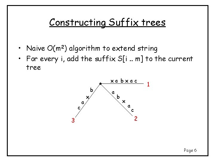
Constructing Suffix trees • Naive O(m 2) algorithm to extend string • For every i, add the suffix S[i. . m] to the current tree xa bxac c 3 a x b a b x a 1 c 2 Page 6

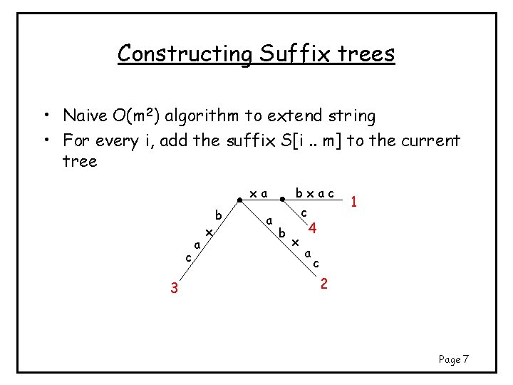
Constructing Suffix trees • Naive O(m 2) algorithm to extend string • For every i, add the suffix S[i. . m] to the current tree xa c 3 a x b a bxac c b x 1 4 a c 2 Page 7

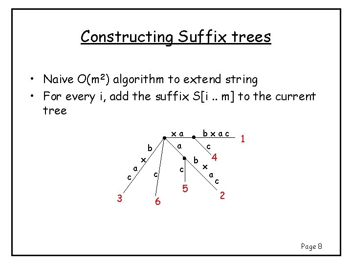
Constructing Suffix trees • Naive O(m 2) algorithm to extend string • For every i, add the suffix S[i. . m] to the current tree c 3 a x xa a b c 6 c 5 bxac c b x 1 4 a c 2 Page 8

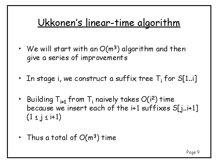
Ukkonen’s linear-time algorithm • We will start with an O(m 3) algorithm and then give a series of improvements • In stage i, we construct a suffix tree Ti for S[1. . i] • Building Ti+1 from Ti naively takes O(i 2) time because we insert each of the i+1 suffixes S[j. . i+1] (1 ≤ j ≤ i+1) • Thus a total of O(m 3) time Page 9

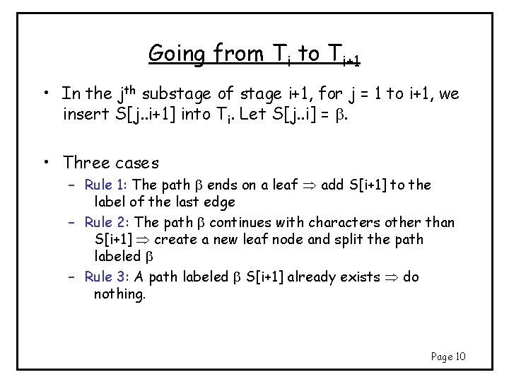
Going from Ti to Ti+1 • In the jth substage of stage i+1, for j = 1 to i+1, we insert S[j. . i+1] into Ti. Let S[j. . i] = b. • Three cases – Rule 1: The path b ends on a leaf add S[i+1] to the label of the last edge – Rule 2: The path b continues with characters other than S[i+1] create a new leaf node and split the path labeled b – Rule 3: A path labeled b S[i+1] already exists do nothing. Page 10

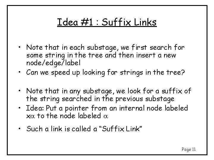
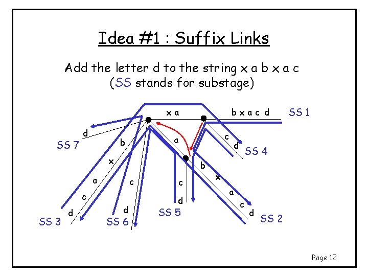
Idea #1 : Suffix Links • Note that in each substage, we first search for some string in the tree and then insert a new node/edge/label • Can we speed up looking for strings in the tree? • Note that in any substage, we look for a suffix of the string searched in the previous substage • Idea: Put a pointer from an internal node labeled xa to the node labeled a • Such a link is called a “Suffix Link” Page 11

Idea #1 : Suffix Links Add the letter d to the string x a b x a c (SS stands for substage) xa SS 7 d c a b x b a c c SS 3 d bxac d d SS 6 c d SS 5 d SS 1 SS 4 x a c d SS 2 Page 12

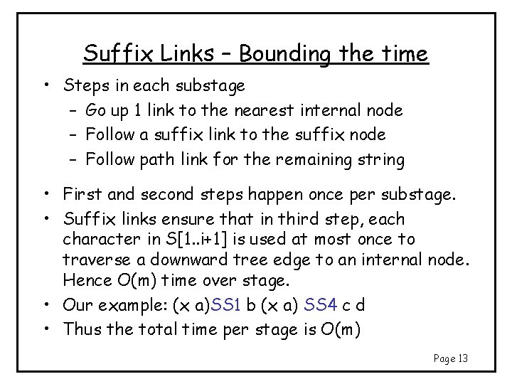
Suffix Links – Bounding the time • Steps in each substage – Go up 1 link to the nearest internal node – Follow a suffix link to the suffix node – Follow path link for the remaining string • First and second steps happen once per substage. • Suffix links ensure that in third step, each character in S[1. . i+1] is used at most once to traverse a downward tree edge to an internal node. Hence O(m) time over stage. • Our example: (x a)SS 1 b (x a) SS 4 c d • Thus the total time per stage is O(m) Page 13

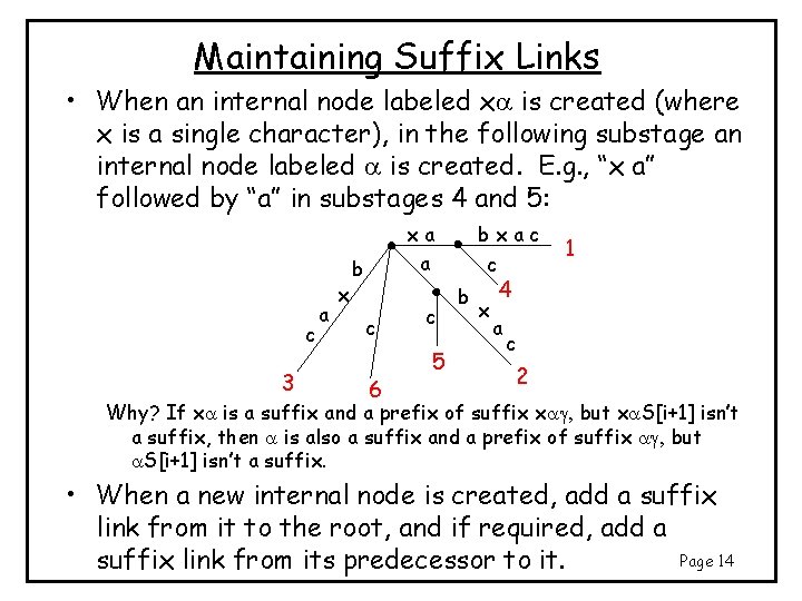
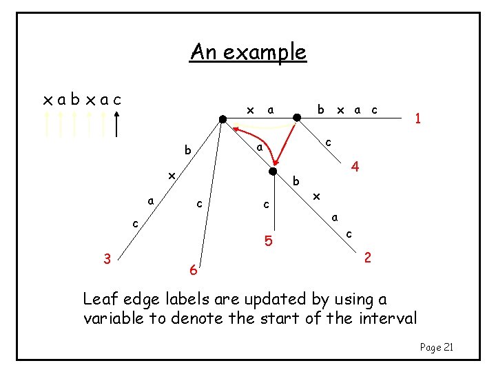
Maintaining Suffix Links • When an internal node labeled xa is created (where x is a single character), in the following substage an internal node labeled a is created. E. g. , “x a” followed by “a” in substages 4 and 5: c 3 a x xa a b c 6 c 5 bxac c b x 1 4 a c 2 Why? If xa is a suffix and a prefix of suffix xa , but xa. S[i+1] isn’t a suffix, then a is also a suffix and a prefix of suffix a , but a. S[i+1] isn’t a suffix. • When a new internal node is created, add a suffix link from it to the root, and if required, add a Page 14 suffix link from its predecessor to it.

Going from O(m 2) to O(m) • Can we even hope to do better than O(m 2)? • Size of the tree itself can be O(m 2) as shown so far • But notice that there at most 2 m edges! Why? (at most m leaves, and all internal nodes have at least two children) (still O(m) even if we double count edges for all suffixes that are prefixes of other suffixes) • Idea: represent labels of edges as intervals • Can easily modify the entire process to work on intervals Page 15

Idea #2 : Getting rid of Rule 3 • Recall Rule 3: A path labeled S[j. . i+1] already exists ) do nothing. • If S[j. . i+1] already exists, then S[j+1. . i+1] exists too and we will again apply Rule 3 in the next substage • Whenever we encounter Rule 3, this stage is over – skip to the next stage. Page 16

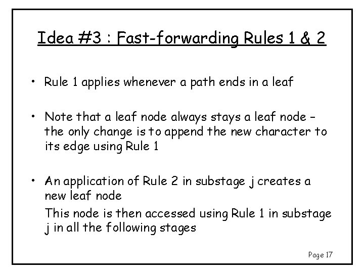
Idea #3 : Fast-forwarding Rules 1 & 2 • Rule 1 applies whenever a path ends in a leaf • Note that a leaf node always stays a leaf node – the only change is to append the new character to its edge using Rule 1 • An application of Rule 2 in substage j creates a new leaf node This node is then accessed using Rule 1 in substage j in all the following stages Page 17

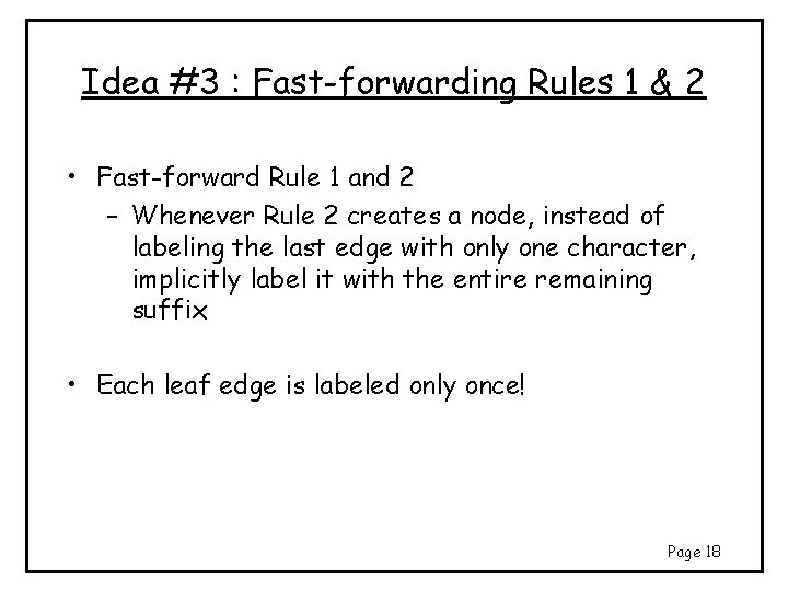
Idea #3 : Fast-forwarding Rules 1 & 2 • Fast-forward Rule 1 and 2 – Whenever Rule 2 creates a node, instead of labeling the last edge with only one character, implicitly label it with the entire remaining suffix • Each leaf edge is labeled only once! Page 18

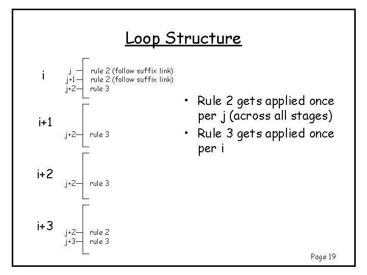
Loop Structure i i+1 i+2 i+3 j j+1 j+2 rule 2 (follow suffix link) rule 3 j+2 j+3 rule 2 rule 3 • Rule 2 gets applied once per j (across all stages) • Rule 3 gets applied once per i Page 19

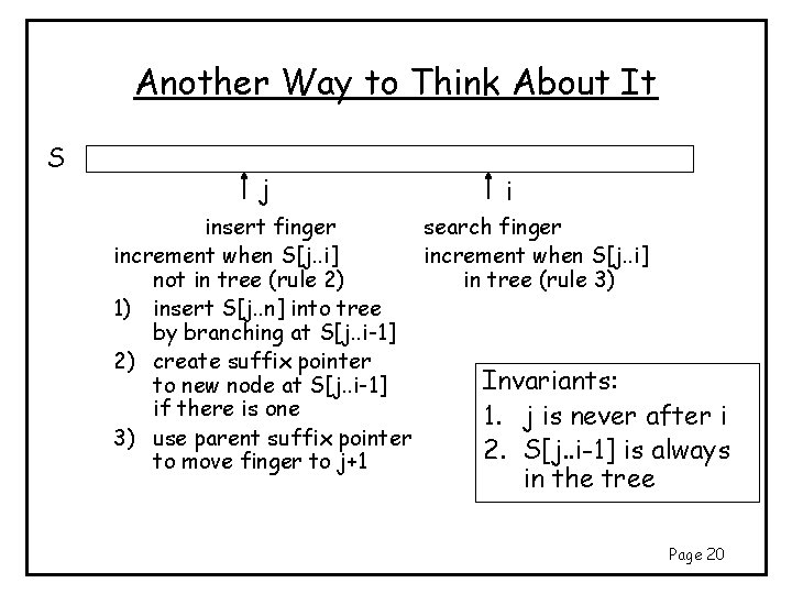
Another Way to Think About It S j i insert finger search finger increment when S[j. . i] not in tree (rule 2) in tree (rule 3) 1) insert S[j. . n] into tree by branching at S[j. . i-1] 2) create suffix pointer Invariants: to new node at S[j. . i-1] if there is one 1. j is never after i 3) use parent suffix pointer 2. S[j. . i-1] is always to move finger to j+1 in the tree Page 20

An example xabxac a x x b c c 3 c 5 6 x a c 1 c a b 4 x a c 2 Leaf edge labels are updated by using a variable to denote the start of the interval Page 21

Complexity Analysis • Rule 3 is used only once in every stage • For every j, Rule 1 & 2 are applied only once in the jth substage of all the stages. • Each application of a rule takes O(1) steps • Other overheads are O(1) per stage • Total time is O(m) Page 22

Extending to multiple texts • Suppose we want to match a pattern with a dictionary of k texts of length m 1, …, mk • Concatenate all the texts (separated by special characters) and construct a common suffix tree • Time taken = O(m 1+…+mk) • Unnecessarily complicated tree; needs special characters Page 23

Multiple texts – Better algorithm • First construct a suffix tree on the first text, then insert suffixes of the second text and so on • Each leaf node should store values corresponding to each text • O(m 1+…+mk) as before Page 24

Longest Common Substring • Find the longest string that is a substring of both text S 1 and text S 2 • Construct a common suffix tree for both texts • Any node that has in its subtree at least one leaf node labeled by S 1 and at least one leaf node labeled by S 2 yields a common substring • The “deepest” such node is the required substring • Can be found in linear time by a tree traversal Page 25

Common substrings of M strings • Given M strings of total length n, find for every k, the length lk of the longest string that is a substring of at least k of the strings • Construct a common suffix tree – O(n) time • For every internal node, find the number of distinctly labeled leaves in the subtree rooted at the node – might take O(Mn) time – not linear! • Report lk by a single tree traversal Page 26

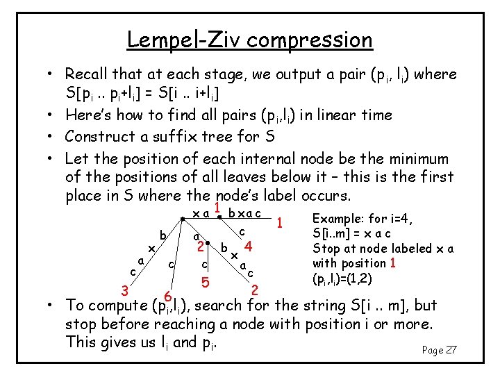
Lempel-Ziv compression • Recall that at each stage, we output a pair (pi, li) where S[pi. . pi+li] = S[i. . i+li] • Here’s how to find all pairs (pi, li) in linear time • Construct a suffix tree for S • Let the position of each internal node be the minimum of the positions of all leaves below it – this is the first place in S where the node’s label occurs. c 3 a x b c 6 x a 1 b xa c c a 2 b 4 x c a c 5 2 1 Example: for i=4, S[i. . m] = x a c Stop at node labeled x a with position 1 (pi, li)=(1, 2) • To compute (pi, li), search for the string S[i. . m], but stop before reaching a node with position i or more. This gives us li and pi. Page 27