Stato dei lavori Ottimizzazione dei wiggler di DAFNE

Stato dei lavori Ottimizzazione dei wiggler di DAFNE Simona Bettoni

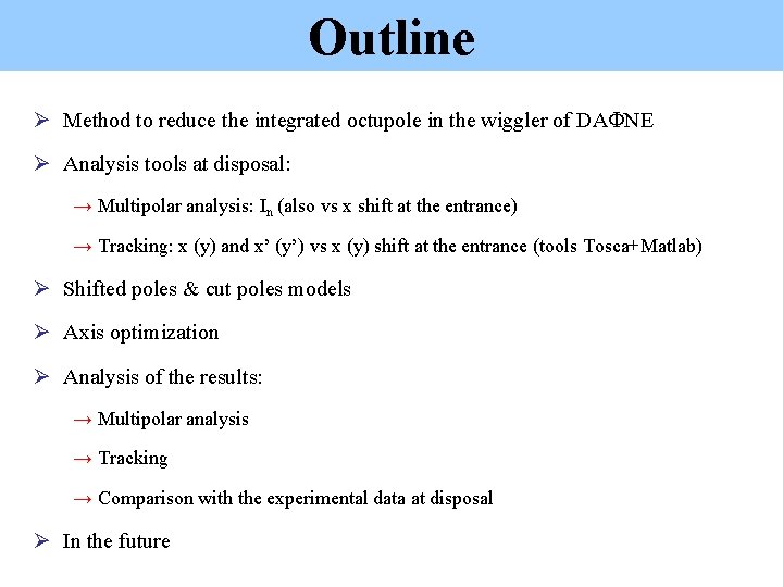
Outline Ø Method to reduce the integrated octupole in the wiggler of DAFNE Ø Analysis tools at disposal: → Multipolar analysis: In (also vs x shift at the entrance) → Tracking: x (y) and x’ (y’) vs x (y) shift at the entrance (tools Tosca+Matlab) Ø Shifted poles & cut poles models Ø Axis optimization Ø Analysis of the results: → Multipolar analysis → Tracking → Comparison with the experimental data at disposal Ø In the future

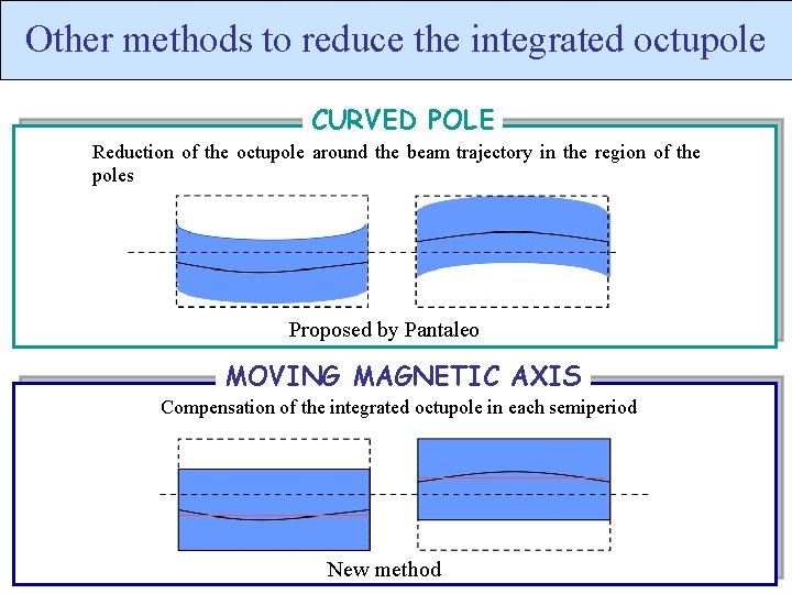
Other methods to reduce the integrated octupole CURVED POLE Reduction of the octupole around the beam trajectory in the region of the poles Proposed by Pantaleo MOVING MAGNETIC AXIS Compensation of the integrated octupole in each semiperiod New method

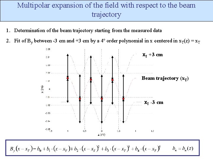
Multipolar expansion of the field with respect to the beam trajectory 1. Determination of the beam trajectory starting from the measured data 2. Fit of By between -3 cm and +3 cm by a 4º order polynomial in x centered in x. T(z) = x. T +3 cm Beam trajectory (x. T) x. T -3 cm

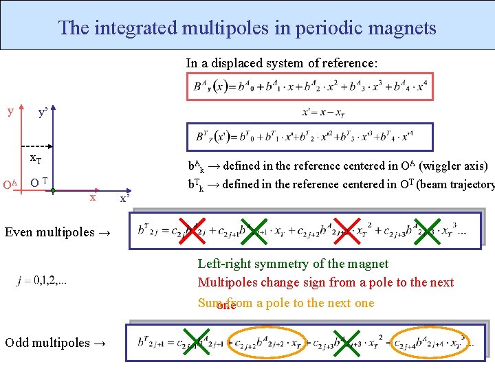
The integrated multipoles in periodic magnets In a displaced system of reference: y y’ x. T OA b. Ak → defined in the reference centered in OA (wiggler axis) OT x x’ b. Tk → defined in the reference centered in OT (beam trajectory Even multipoles → Left-right symmetry of the magnet Multipoles change sign from a pole to the next Sumone from a pole to the next one Odd multipoles →

Method to reduce the integrated octupole: displacement of the magnetic field WITHOUT POLE MODIFICATION In each semiperiod the particle trajectory is always on one side with respect the magnetic axis ↑ Octupole WITH THE POLE MODIFICATION In each semiperiod the particle travels on both sides with respect to the magnetic axis Opportunely choosing the B axis is in principle possible to make zero the integrated octupole in each semiperiod

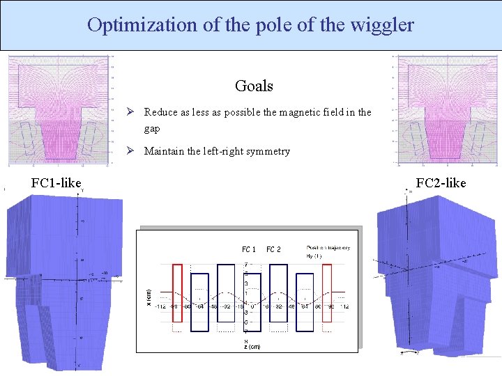
Optimization of the pole of the wiggler Goals Ø Reduce as less as possible the magnetic field in the gap Ø Maintain the left-right symmetry FC 1 -like FC 2 -like FC 1 FC 2

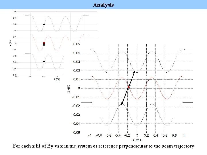
Analysis For each z fit of By vs x in the system of reference perpendicular to the beam trajectory

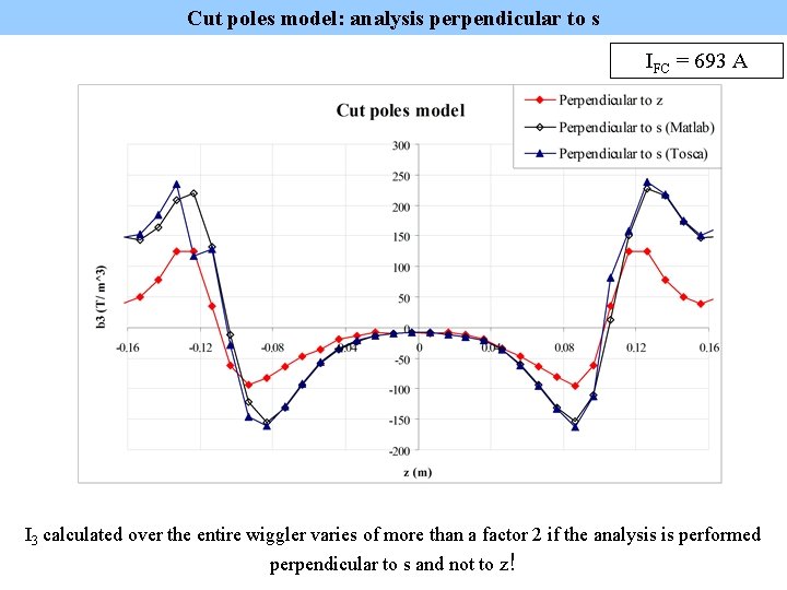
Cut poles model: analysis perpendicular to s IFC = 693 A I 3 calculated over the entire wiggler varies of more than a factor 2 if the analysis is performed perpendicular to s and not to z!

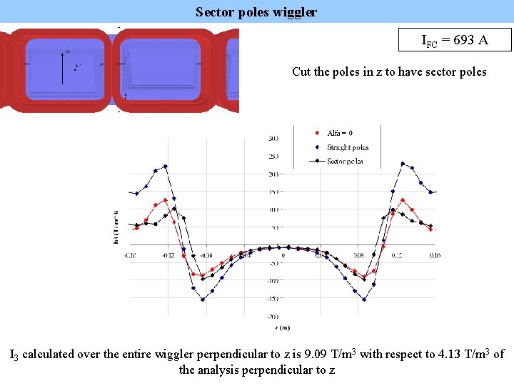
Sector poles wiggler IFC = 693 A Cut the poles in z to have sector poles I 3 calculated over the entire wiggler perpendicular to z is 9. 09 T/m 3 with respect to 4. 13 T/m 3 of the analysis perpendicular to z

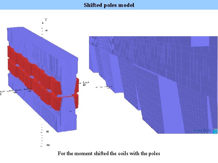
Shifted poles solution $ and field rolloff

Shifted poles model For the moment shifted the coils with the poles

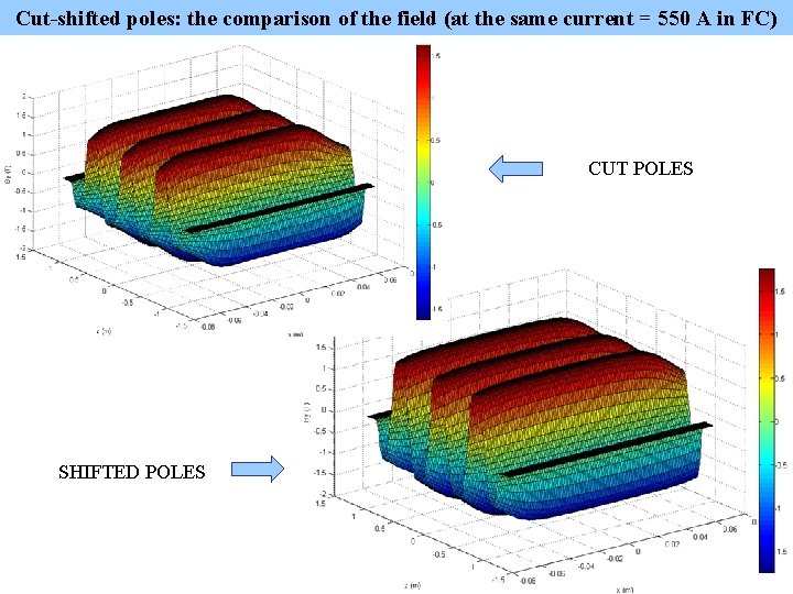
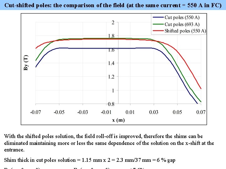
Cut-shifted poles: the comparison of the field (at the same current = 550 A in FC) CUT POLES SHIFTED POLES

Cut-shifted poles: the comparison of the field (at the same current = 550 A in FC) With the shifted poles solution, the field roll-off is improved, therefore the shims can be eliminated maintaining more or less the same dependence of the solution on the x-shift at the entrance. Shim thick in cut poles solution = 1. 15 mm x 2 = 2. 3 mm/37 mm = 6 % gap

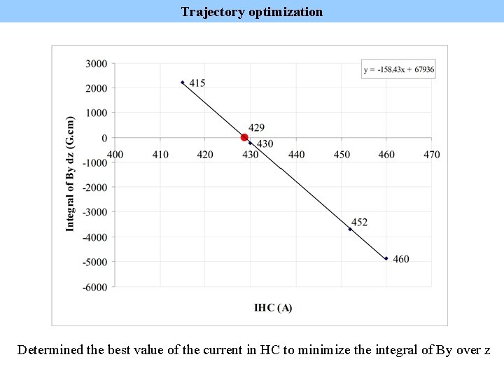
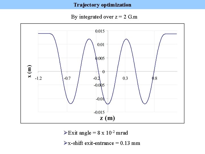
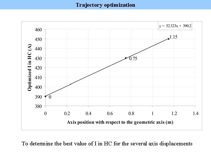
Trajectory optimization Determined the best value of the current in HC to minimize the integral of By over z

Trajectory optimization By integrated over z = 2 G. m ØExit angle = 8 x 10 -2 mrad Øx-shift exit-entrance = 0. 13 mm

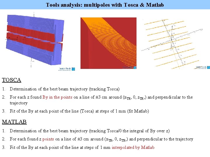
Tools analysis: multipoles with Tosca & Matlab TOSCA 1. Determination of the best beam trajectory (tracking Tosca) 2. For each z found By in the points on a line of ± 3 cm around (x. TR, 0, z. TR, ) and perpendicular to the trajectory 3. Fit of the By at each point of the line (Tosca) at steps of 1 mm (fit Matlab) MATLAB 1. Determination of the best beam trajectory (tracking Tosca/0 the integral of By over z) 2. For each found z points on a line of ± 3 cm around (x. TR, 0, z. TR, ) and perpendicular to the trajectory 3. Fit of the By at each point of the line at steps of 1 mm interpolated by Matlab

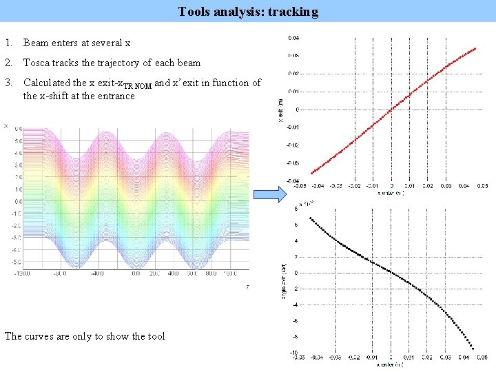
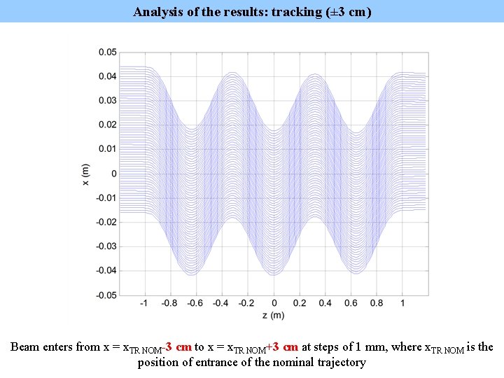
Tools analysis: tracking 1. Beam enters at several x 2. Tosca tracks the trajectory of each beam 3. Calculated the x exit-x. TR NOM and x’exit in function of the x-shift at the entrance The curves are only to show the tool

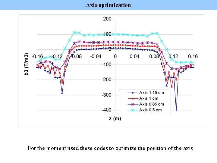
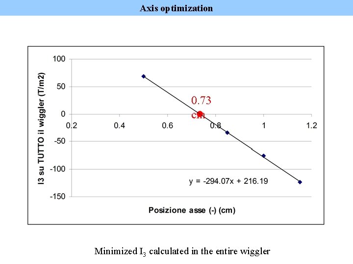
Axis optimization For the moment used these codes to optimize the position of the axis

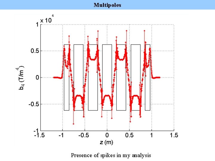
Multipoles Presence of spikes in my analysis

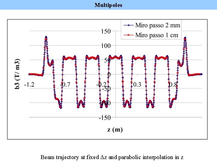
Multipoles Beam trajectory at fixed Dz and parabolic interpolation in z

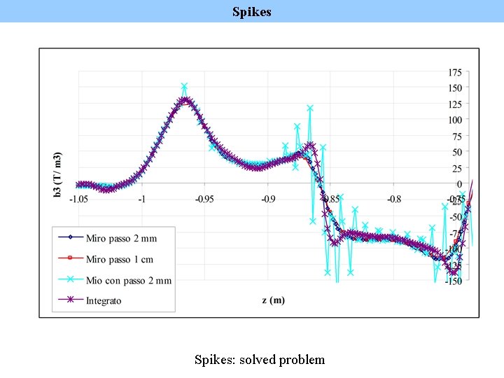
Spikes: solved problem

Axis optimization 0. 73 cm Minimized I 3 calculated in the entire wiggler

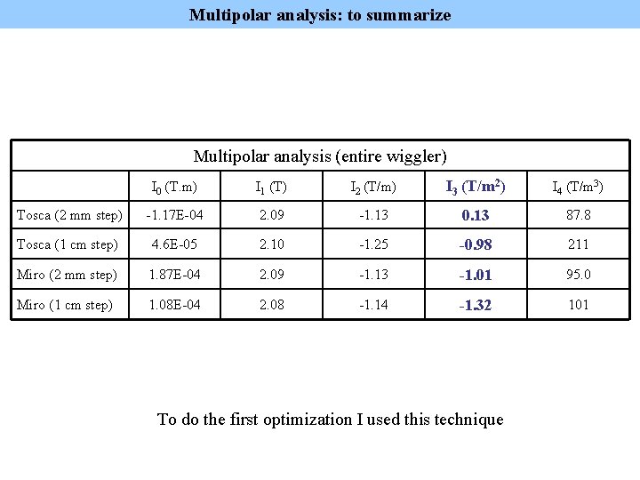
Multipolar analysis: to summarize Multipolar analysis (entire wiggler) I 0 (T. m) I 1 (T) I 2 (T/m) I 3 (T/m 2) I 4 (T/m 3) Tosca (2 mm step) -1. 17 E-04 2. 09 -1. 13 0. 13 87. 8 Tosca (1 cm step) 4. 6 E-05 2. 10 -1. 25 -0. 98 211 Miro (2 mm step) 1. 87 E-04 2. 09 -1. 13 -1. 01 95. 0 Miro (1 cm step) 1. 08 E-04 2. 08 -1. 14 -1. 32 101 To do the first optimization I used this technique

Analysis of the results: tracking (± 3 cm) Beam enters from x = x. TR NOM-3 cm to x = x. TR NOM+3 cm at steps of 1 mm, where x. TR NOM is the position of entrance of the nominal trajectory

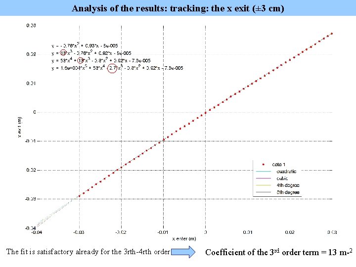
Analysis of the results: tracking: the x exit (± 3 cm) The fit is satisfactory already for the 3 rth-4 rth order Coefficient of the 3 rd order term = 13 m-2

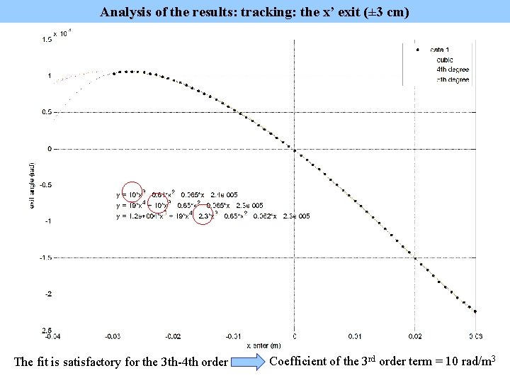
Analysis of the results: tracking: the x’ exit (± 3 cm) The fit is satisfactory for the 3 th-4 th order Coefficient of the 3 rd order term = 10 rad/m 3

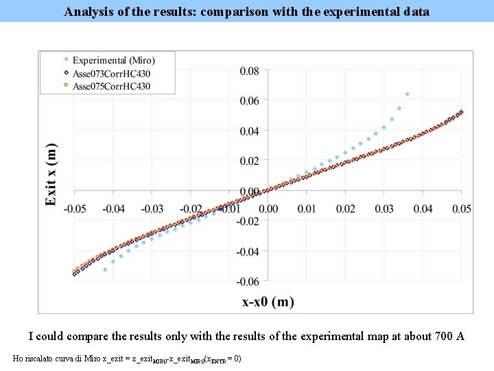
Analysis of the results: comparison with the experimental data I could compare the results only with the results of the experimental map at about 700 A Ho riscalato curva di Miro x_exit = x_exit. MIRO-x_exit. MIRO(x. ENTR = 0)

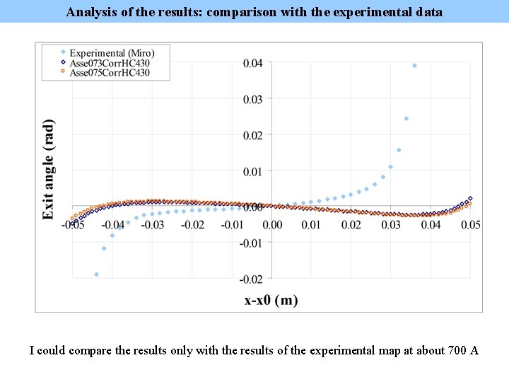
Analysis of the results: comparison with the experimental data I could compare the results only with the results of the experimental map at about 700 A

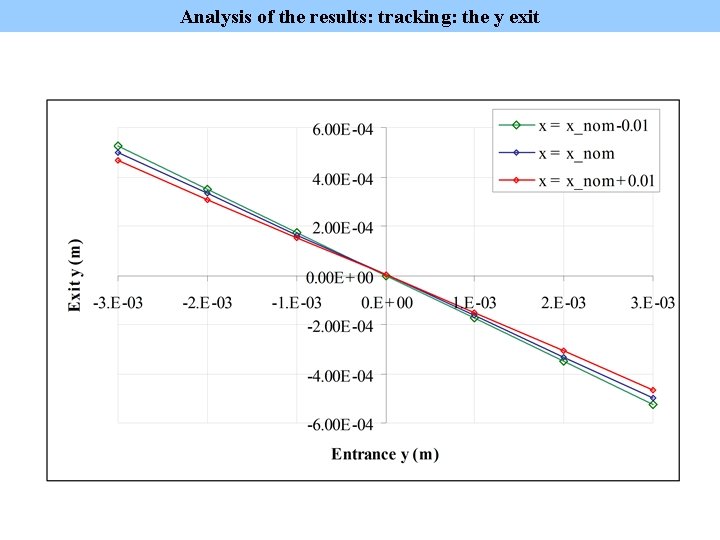
Analysis of the results: tracking: the y exit

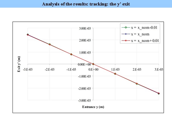
Analysis of the results: tracking: the y’ exit

Conclusions Ø Shifted poles - cut poles solution comparison: Ø The field roll-off is improved no shim increased BPEAK Ø Cheaper Ø At present: è improved the linearity zone of x and x’ with respect to the field map at dipsosal Ø In the future: è Shifted poles solution analysis: Analysis of the field maps by Dragt, Mitchell and Venturini (the map considered the best one by us, one with the poles more centered and one with the poles more shifted) è Measurement of the field map of the wiggler at I = 550 A to have a real comparison with the results of the simulation (at LNF, at ENEA? )

Di scorta…

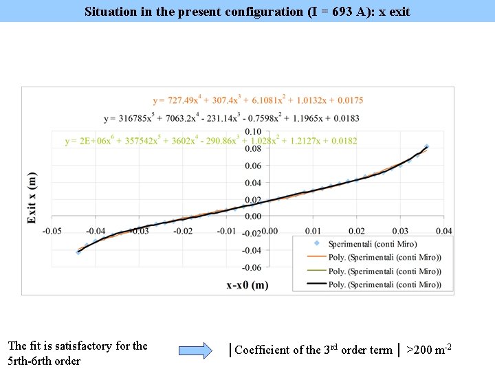
Situation in the present configuration (I = 693 A): x exit The fit is satisfactory for the 5 rth-6 rth order │Coefficient of the 3 rd order term │ >200 m-2

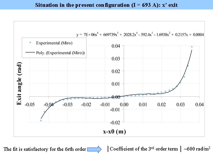
Situation in the present configuration (I = 693 A): x’ exit The fit is satisfactory for the 6 rth order │Coefficient of the 3 rd order term │ ~600 rad/m 3

Trajectory optimization To determine the best value of I in HC for the several axis displacements

Fine!