Statistical inference Hypothesis testing Claudia von Brmssen Hypothesis

Statistical inference Hypothesis testing Claudia von Brömssen

Hypothesis testing Example: The milk yield of a new breed is examined. It is interesting to know if the average yield is significantly above 25 kg/ day. 10 observations are collected.

Hypothesis testing To be able to conduct a statistical test we need: • Two hypotheses H 0 (nullhypotesis): is to be ‘proved’ wrong H 1 (alternative hypotesis): to be ‘proved’ • • A point estimate of the measure we want to examine The standard error of the point estimate The distribution of the point estimate The signifikance level a, which is determined by the user, often 5% or 1%

The distribution is centered around the value in the null hypothesis (which here is also the unknown population mean, since the null hypothesis is assumed to be true).

Hypothesis testing: Principles General question: How ‘extreme’ is the observed mean in comparison to the distribution on the last slide? Is it among the most extreme cases = the tails of the distribution? If is among the most extreme 5% -> we reject the null hypothesis = we do not believe the null hypothesis is true.
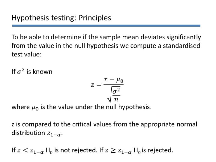

Hypothesis testing: Principles The sample mean is checked against the critical value (here the upper 5% of the distribution, the 95% quantile):

Example: Milk yield

One- and two-tailed tests: We have conducted one tailed test, where we only are interested if the milk yield is larger than 25 kg/day. Another possibility is to conduct a one-sided test to check if the milk yield is significantly less than 25 kg/day.

One- and two-tailed tests: In many contexts it is most interesting to test both sides, i. e. to detect if the true mean is either less than or larger than the hypothised value: a two-tailed test is used.
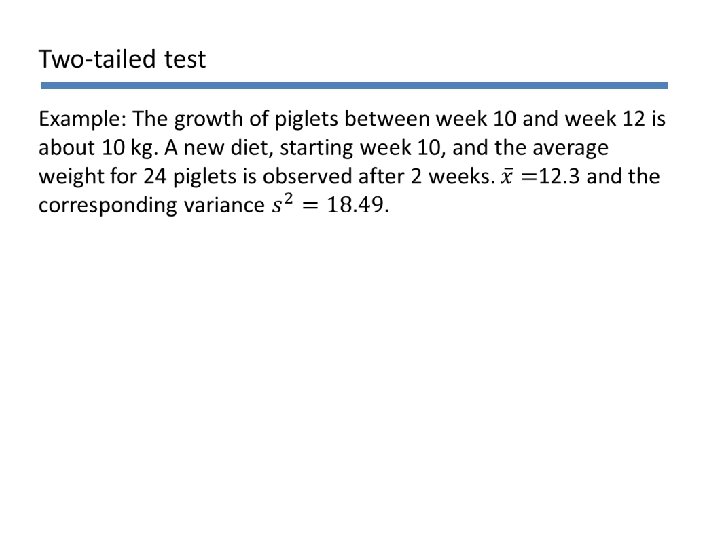
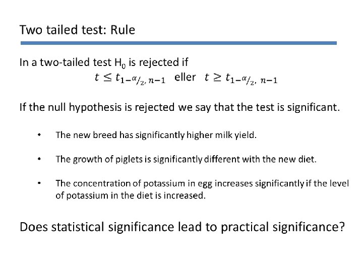

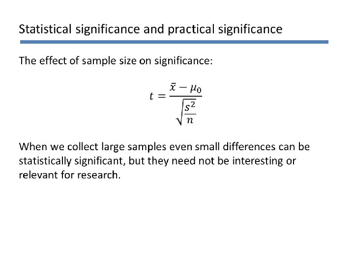
Statistical significance and practical significance When we have made a conclusion in a statistical test we also need to evaluate this conclusion within our area of application. The weight of a piglet increases with is 2. 3 kg compared to standard diets: Is that a lot/important/interesting? What about an increase of 0. 2 kg?

P-value When the analysis is done with a computer program the z-test or t-test are presented with a p-value. Example: milk yield: the sample mean was 25. 98 The probability to get the observed value of an even more extreme value is called the p-value. For the example: p= 0. 06167

P-value The p-value is compared with the significance level. If the p-value is less then the significance level the null hypothesis H 0 is rejected. Example: Milk yield P-value: Significance level: Conclusion:
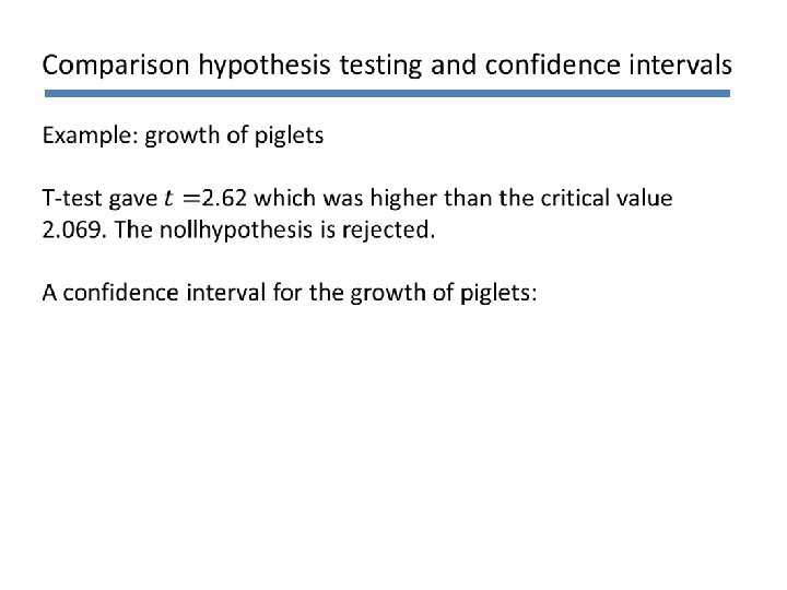

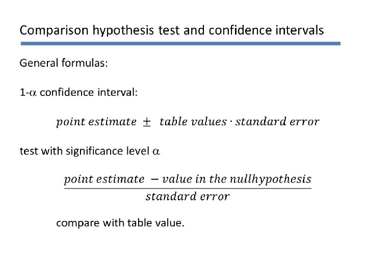
Comparison of hypothesis tests and confidence intervals Confidence intervals can be used to conduct hypothesis testing if both are of the same type (one-tailed, two-tailed) have the same level a (a = significance level , 1 a = confidence level) There are tests that do not have a corresponding confidence interval.

Errors in statistical tests Hypothesis tests are based on probabilities and are never certain. We decide the significance level or confidence level which determine the level of certainty. In a statistical test we do either reject or not reject the nullhypothesis. If the observed value is not probable under the nullhypothesis we reject this hypothesis (we believe it wrong).

Errors in statistical tests

Error in statistical tests Error of the first kind – Type I error: If the null hypothesis is true, but the test rejects it. The probability of this error is decided by the significance level. The probability of this error is a.

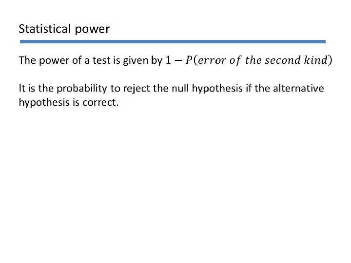
Error in statistical tests Error of the second kind – Type II error: If the null hypothesis is wrong, but the test does not reject it The probability for this error can be computed from • the significance level a, • the sample size n and • how wrong the nullhypothesis is. Black line =critical value Do not reject H 0 Reject H 0

Power curves for different sample sizes - the more observations the larger the power to detect even small differences.

How to check is datasets are normally distributed QQplots: Not normally distributed Normally distributed

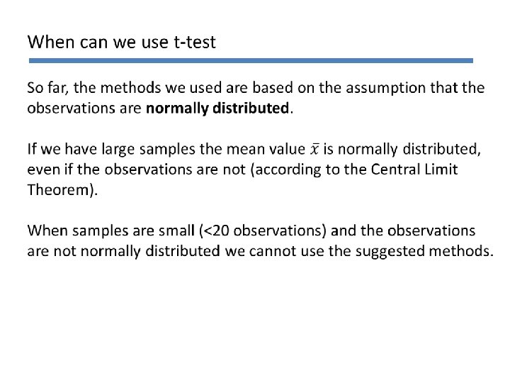
Non-parametric methods: Assumptions Observe that nonparametric methods here relax the assumption of normality. Any distribution of data is fine. Observations need however still be independent. Nonparametric methods are not a magical tool that work for anything, but have important restrictions too.

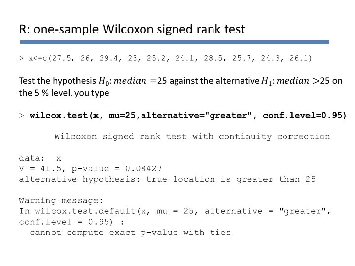
Non-parametric methods: The signed rank test To compute a signed rank test the observations are replaced with their ranks. The test still assumes that the distribution of the observation is symmetric, but it does not need to be normally distributed. No handcalculations for non-parametric methods in this course, but we use them in the computer exercises.
 One Sample t-test data: x t")
> t. test(x, mu=25, alternative="greater", conf. level=0. 95) One Sample t-test data: x t = 1. 5432, df = 9, p-value = 0. 07859 alternative hypothesis: true mean is greater than 25 95 percent confidence interval: 24. 81588 Inf sample estimates: mean of x 25. 98

SAS: read data milkyield; input yield; cards; 27. 5 26 29. 4 23 25. 2 24. 1 28. 5 25. 7 24. 3 26. 1 ; run;
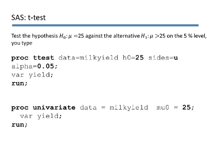

SAS: t-test The TTEST Procedure Variable: N 10 Mean 25. 9800 Std Dev 2. 0082 95% CL Mean 24. 8159 Infty DF 9 yield Std Err 0. 6351 Minimum 23. 0000 Std Dev 2. 0082 t Value 1. 54 Pr > t 0. 0786 Maximum 29. 4000 95% CL Std Dev 1. 3813 3. 6662
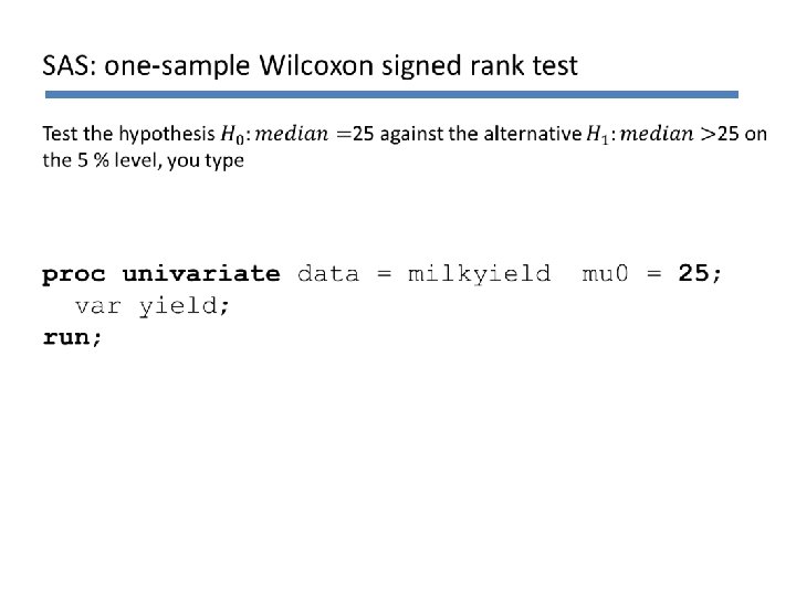

SAS: one-sample Wilcoxon signed rank test The UNIVARIATE Procedure Variable: yield Tests for Location: Mu 0=25 Test -Statistic- -----p Value------ Student's t Signed Rank t M S Pr > |t| Pr >= |M| Pr >= |S| 1. 543185 2 14 0. 1572 0. 3438 0. 1680 Quantiles (Definition 5) Level 100% Max 99% 95% 90% 75% Q 3 Quantile 29. 40 28. 95 27. 50 Tests are always two-sided.
- Slides: 37