Statistical Hypothesis Testing Review q A statistical hypothesis

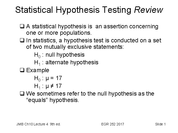
Statistical Hypothesis Testing Review q A statistical hypothesis is an assertion concerning one or more populations. q In statistics, a hypothesis test is conducted on a set of two mutually exclusive statements: H 0 : null hypothesis H 1 : alternate hypothesis q Example H 0 : μ = 17 H 1 : μ ≠ 17 q We sometimes refer to the null hypothesis as the “equals” hypothesis. JMB Ch 10 Lecture 4 9 th ed. EGR 252 2017 Slide 1

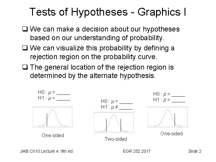
Tests of Hypotheses - Graphics I q We can make a decision about our hypotheses based on our understanding of probability. q We can visualize this probability by defining a rejection region on the probability curve. q The general location of the rejection region is determined by the alternate hypothesis. H 0 : μ = _____ H 1 : μ < _____ One-sided JMB Ch 10 Lecture 4 9 th ed. H 0 : μ = _____ H 1 : μ ≠ _____ H 0 : p = _____ H 1 : p > _____ One-sided Two-sided EGR 252 2017 Slide 2

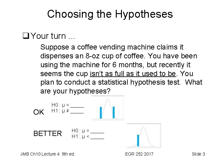
Choosing the Hypotheses q Your turn … Suppose a coffee vending machine claims it dispenses an 8 -oz cup of coffee. You have been using the machine for 6 months, but recently it seems the cup isn’t as full as it used to be. You plan to conduct a statistical hypothesis test. What are your hypotheses? OK H 0 : μ = _____ H 1 : μ ≠ _____ BETTER H 0 : μ = _____ H 1 : μ < _____ JMB Ch 10 Lecture 4 9 th ed. EGR 252 2017 Slide 3

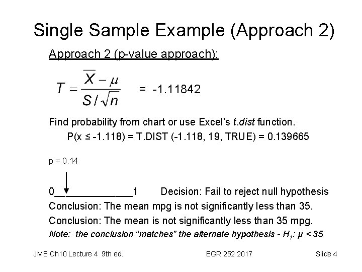
Single Sample Example (Approach 2) Approach 2 (p-value approach): = -1. 11842 Find probability from chart or use Excel’s t. dist function. P(x ≤ -1. 118) = T. DIST (-1. 118, 19, TRUE) = 0. 139665 p = 0. 14 0_______1 Decision: Fail to reject null hypothesis Conclusion: The mean mpg is not significantly less than 35. Conclusion: The mean is not significantly less than 35 mpg. Note: the conclusion “matches” the alternate hypothesis - H 1: μ < 35 JMB Ch 10 Lecture 4 9 th ed. EGR 252 2017 Slide 4

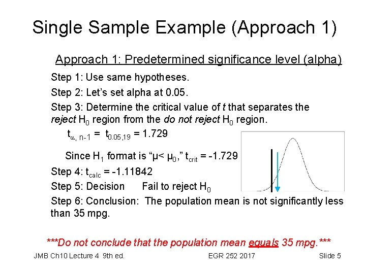
Single Sample Example (Approach 1) Approach 1: Predetermined significance level (alpha) Step 1: Use same hypotheses. Step 2: Let’s set alpha at 0. 05. Step 3: Determine the critical value of t that separates the reject H 0 region from the do not reject H 0 region. t , n-1 = t 0. 05, 19 = 1. 729 Since H 1 format is “μ< μ 0, ” tcrit = -1. 729 Step 4: tcalc = -1. 11842 Step 5: Decision Fail to reject H 0 Step 6: Conclusion: The population mean is not significantly less than 35 mpg. ***Do not conclude that the population mean equals 35 mpg. *** JMB Ch 10 Lecture 4 9 th ed. EGR 252 2017 Slide 5

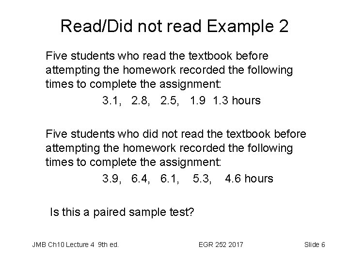
Read/Did not read Example 2 Five students who read the textbook before attempting the homework recorded the following times to complete the assignment: 3. 1, 2. 8, 2. 5, 1. 9 1. 3 hours Five students who did not read the textbook before attempting the homework recorded the following times to complete the assignment: 3. 9, 6. 4, 6. 1, 5. 3, 4. 6 hours Is this a paired sample test? JMB Ch 10 Lecture 4 9 th ed. EGR 252 2017 Slide 6

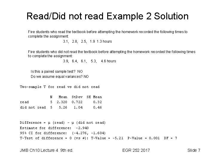
Read/Did not read Example 2 Solution Five students who read the textbook before attempting the homework recorded the following times to complete the assignment: 3. 1, 2. 8, 2. 5, 1. 9 1. 3 hours Five students who did not read the textbook before attempting the homework recorded the following times to complete the assignment: 3. 9, 6. 4, 6. 1, 5. 3, 4. 6 hours Is this a paired sample test? NO Do we assume equal variances? NO Two-sample T for read vs did not read N 5 5 Mean 2. 320 5. 26 St. Dev 0. 722 1. 04 SE Mean 0. 32 0. 46 Difference = μ (read) - μ (did not read) Estimate for difference: -2. 940 95% CI for difference: (-4. 276, -1. 604) T-Test of difference = 0 (vs ≠): T-Value = -5. 21 JMB Ch 10 Lecture 4 9 th ed. P-Value = 0. 001 EGR 252 2017 DF = 7 Slide 7

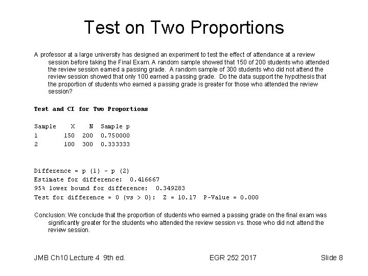
Test on Two Proportions A professor at a large university has designed an experiment to test the effect of attendance at a review session before taking the Final Exam. A random sample showed that 150 of 200 students who attended the review session earned a passing grade. A random sample of 300 students who did not attend the review session showed that only 100 earned a passing grade. Do the data support the hypothesis that the proportion of students who earned a passing grade is greater for those who attended the review session? Test and CI for Two Proportions Sample 1 2 X 150 100 N 200 300 Sample p 0. 750000 0. 333333 Difference = p (1) - p (2) Estimate for difference: 0. 416667 95% lower bound for difference: 0. 349283 Test for difference = 0 (vs > 0): Z = 10. 17 P-Value = 0. 000 Conclusion: We conclude that the proportion of students who earned a passing grade on the final exam was significantly greater for the students who attended the review session vs. those who did not attend the review session. JMB Ch 10 Lecture 4 9 th ed. EGR 252 2017 Slide 8