Stat 155 Section 2 Last Time Continuous Random

Stat 155, Section 2, Last Time • Continuous Random Variables – Probabilities modeled with areas • Normal Curve – Calculate in Excel: NORMDIST & NORMINV • Means, i. e. Expected Values – Useful for “average over many plays” • Independence of Random Variables

Reading In Textbook Approximate Reading for Today’s Material: Pages 277 -286, 291 -305 Approximate Reading for Next Class: Pages 291 -305, 334 -351

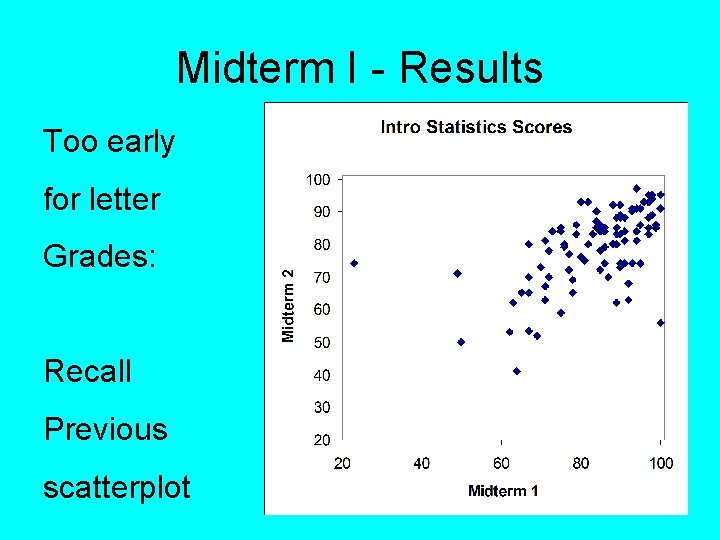
Midterm I - Results Preliminary comments: • Circled numbers are points taken off • Total for each problem in brackets • Points evenly divided among parts • Page total in lower right corner • Check those sum to total on front • Overall score out of 100 points

Midterm I - Results Interpretation of Scores: • Too early for letter grades • These will change a lot: • – Some with good grades will relax – Some with bad grades will wake up Don’t believe “A & C” average to “B”

Midterm I - Results Too early for letter Grades: Recall Previous scatterplot

Midterm I - Results Interpretation of Scores: • 85 – 100 Very Pleased

Midterm I - Results Interpretation of Scores: • 85 – 100 Very Pleased • 65 – 84 OK

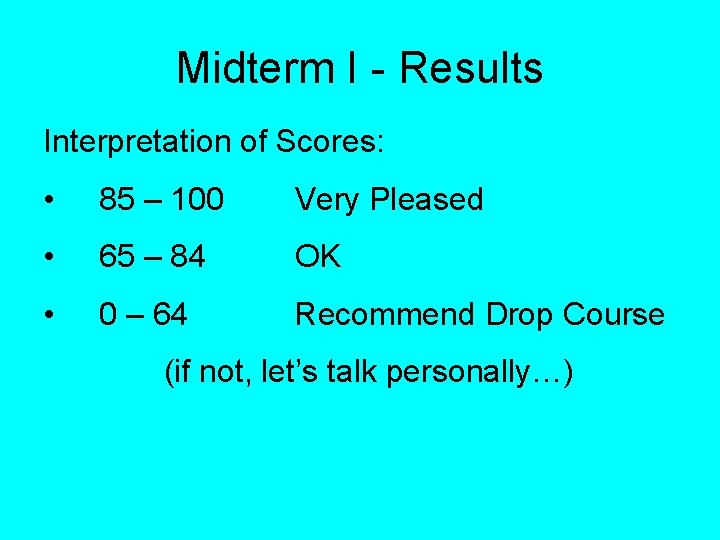
Midterm I - Results Interpretation of Scores: • 85 – 100 Very Pleased • 65 – 84 OK • 0 – 64 Recommend Drop Course (if not, let’s talk personally…)

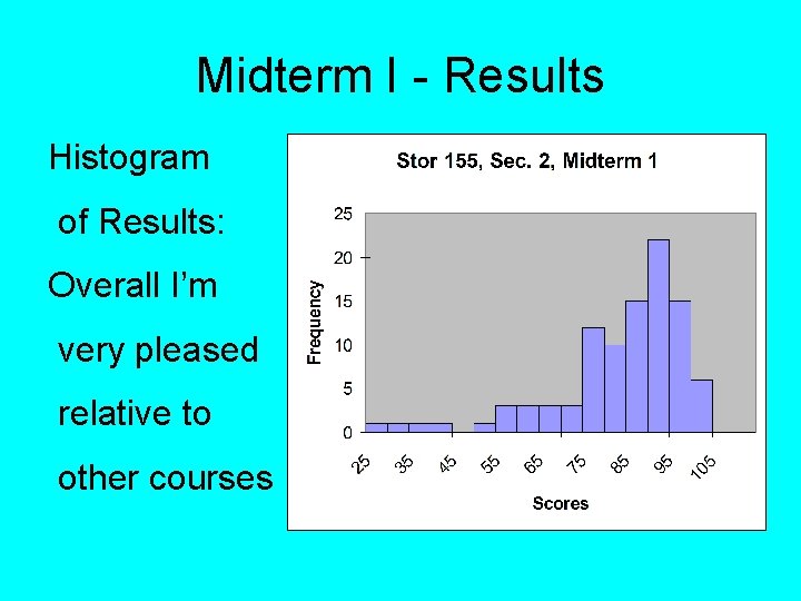
Midterm I - Results Histogram of Results: Overall I’m very pleased relative to other courses

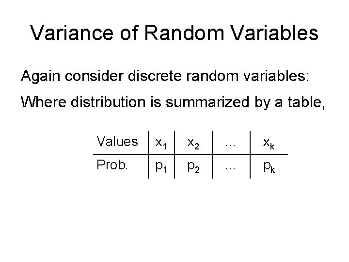
Variance of Random Variables Again consider discrete random variables: Where distribution is summarized by a table, Values x 1 x 2 … xk Prob. p 1 p 2 … pk

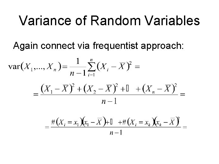
Variance of Random Variables Again connect via frequentist approach:

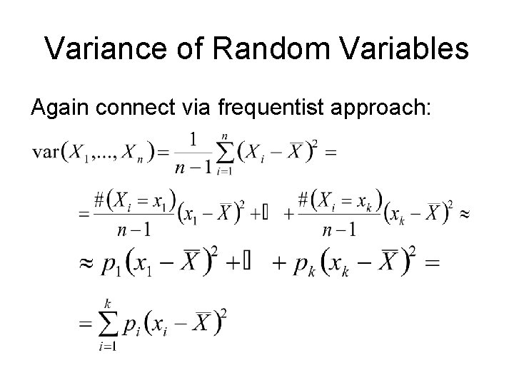
Variance of Random Variables Again connect via frequentist approach:

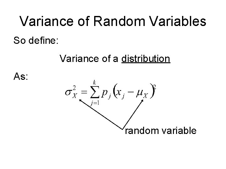
Variance of Random Variables So define: Variance of a distribution As: random variable

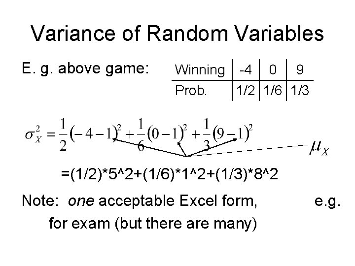
Variance of Random Variables E. g. above game: Winning -4 0 9 Prob. 1/2 1/6 1/3 =(1/2)*5^2+(1/6)*1^2+(1/3)*8^2 Note: one acceptable Excel form, for exam (but there are many) e. g.

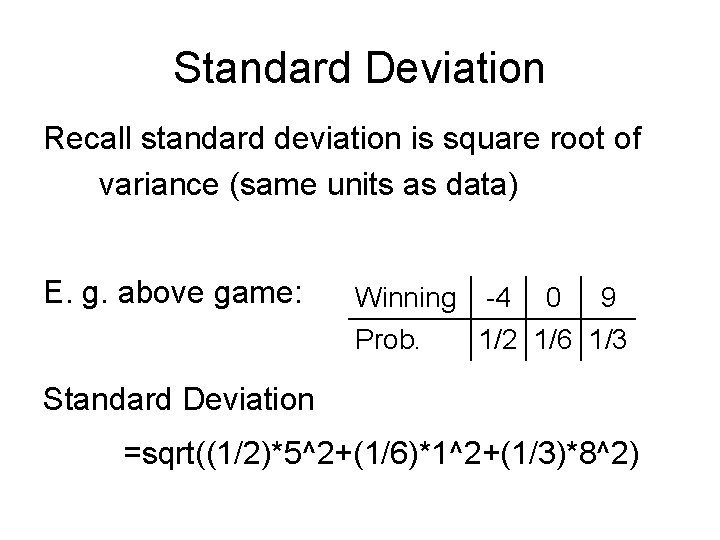
Standard Deviation Recall standard deviation is square root of variance (same units as data) E. g. above game: Winning -4 0 9 Prob. 1/2 1/6 1/3 Standard Deviation =sqrt((1/2)*5^2+(1/6)*1^2+(1/3)*8^2)

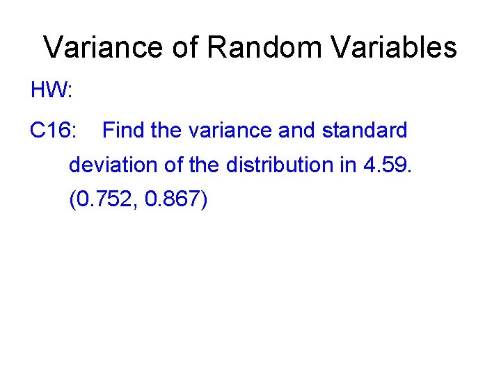
Variance of Random Variables HW: C 16: Find the variance and standard deviation of the distribution in 4. 59. (0. 752, 0. 867)

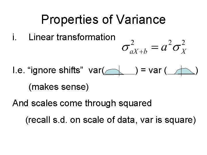
Properties of Variance i. Linear transformation I. e. “ignore shifts” var( ) = var ( ) (makes sense) And scales come through squared (recall s. d. on scale of data, var is square)

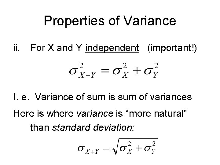
Properties of Variance ii. For X and Y independent (important!) I. e. Variance of sum is sum of variances Here is where variance is “more natural” than standard deviation:

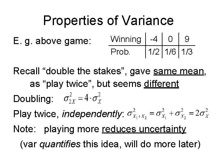
Properties of Variance E. g. above game: Winning -4 0 9 Prob. 1/2 1/6 1/3 Recall “double the stakes”, gave same mean, as “play twice”, but seems different Doubling: Play twice, independently: Note: playing more reduces uncertainty (var quantifies this idea, will do more later)

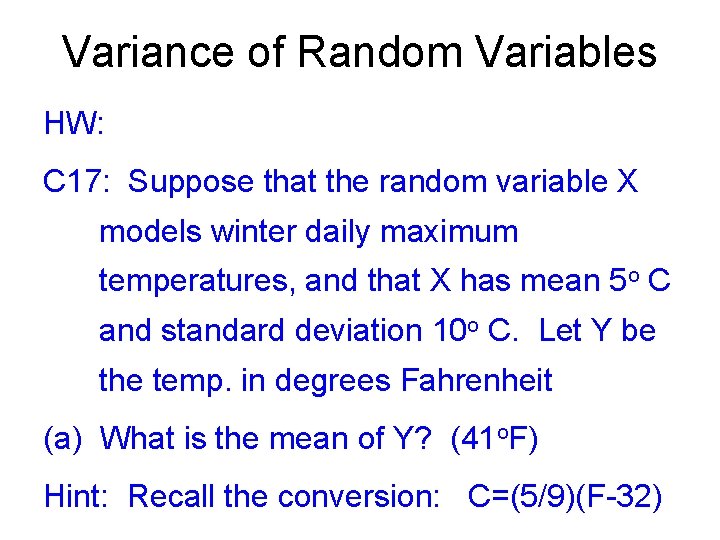
Variance of Random Variables HW: C 17: Suppose that the random variable X models winter daily maximum temperatures, and that X has mean 5 o C and standard deviation 10 o C. Let Y be the temp. in degrees Fahrenheit (a) What is the mean of Y? (41 o. F) Hint: Recall the conversion: C=(5/9)(F-32)

Variance of Random Variables HW: C 17: (cont. ) (b) What is the standard deviation of Y? (18 o. F)

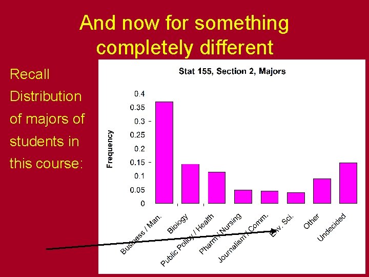
And now for something completely different Recall Distribution of majors of students in this course:

And now for something completely different Couldn’t Find Any Great Jokes, So…

And now for something completely different An Interesting and Relevant Issue: • “Places Rated” • Rankings Published by Several… • We’ve been #1? • Are we great ot what? Will take a careful look later

Chapter 5 Sampling Distributions Idea: Extend probability tools to distributions we care about: (i) Counts in Political Polls (ii) Measurement Error

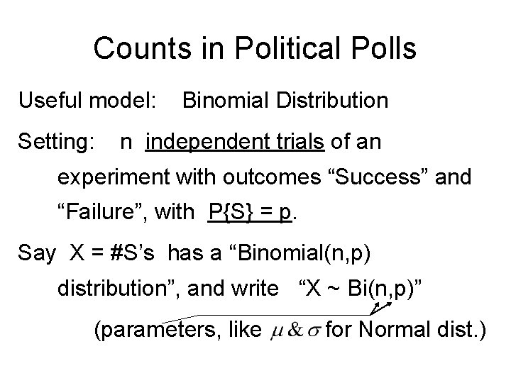
Counts in Political Polls Useful model: Setting: Binomial Distribution n independent trials of an experiment with outcomes “Success” and “Failure”, with P{S} = p. Say X = #S’s has a “Binomial(n, p) distribution”, and write “X ~ Bi(n, p)” (parameters, like for Normal dist. )

Binomial Distributions Models much more than political polls: E. g. Coin tossing (recall saw “independence” was good) E. g. Shooting free throws (in basketball) • Is p always the same? • Really independent? (turns out to be OK)

Binomial Distributions HW on Binomial Assumptions: 5. 1, 5. 2 (a. no, n? , b. yes, c. yes)

Binomial Distributions Could work out a formula for Binomial Probs, but results are summarized in Excel function: BINOMDIST Example of Use: http: //stat-or. unc. edu/webspace/postscript/marron/Teaching/stor 155 -2007/Stor 155 Eg 19. xls

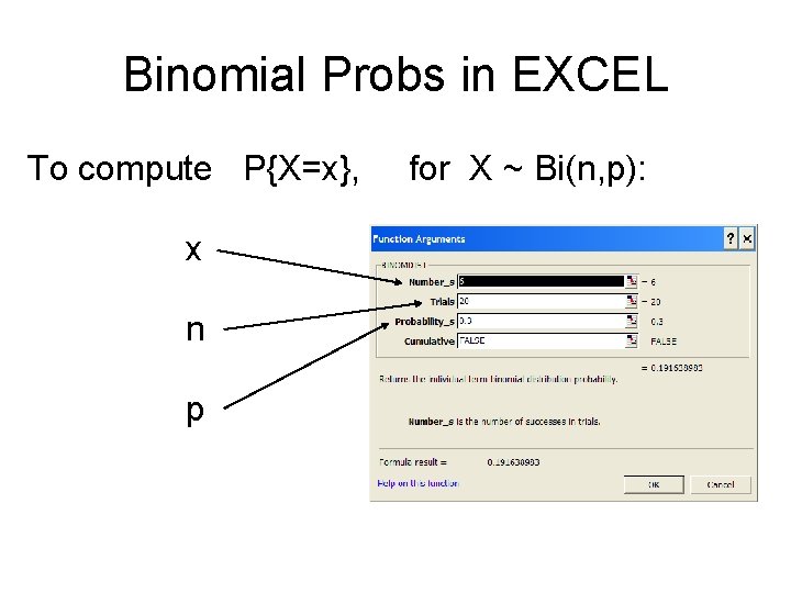
Binomial Probs in EXCEL To compute P{X=x}, x n p for X ~ Bi(n, p):

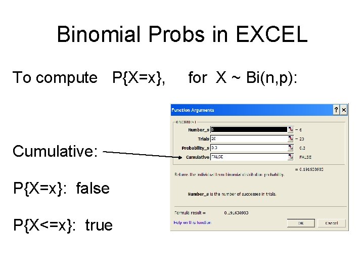
Binomial Probs in EXCEL To compute P{X=x}, Cumulative: P{X=x}: false P{X<=x}: true for X ~ Bi(n, p):

Binomial Probs in EXCEL http: //stat-or. unc. edu/webspace/postscript/marron/Teaching/stor 155 -2007/Stor 155 Eg 19. xls Check this spreadsheet for details of other parts, and some important variations

Binomial Probs in EXCEL Next time: More slides on BINOMDIST, And illustrate things like P{X < 3} = P{X <= 2}, etc. Using a number line, and filled in dots…

Binomial Probs in EXCEL HW: 5. 3 5. 4 (0. 194) Rework, using the Binomial Distribution: 4. 52 c, d

Binomial Distribution “Shape” of Binomial Distribution: Use Probability Histogram Just a bar graph, where heights are probabilities Note: connected to previous histogram by frequentist view (via histogram of repeated samples)

Binomial Distribution Study Distribution Shapes using Excel http: //stat-or. unc. edu/webspace/postscript/marron/Teaching/stor 155 -2007/Stor 155 Eg 20. xls Part I: different p, note several ranges of p are shown Part II: different n, note really “live in different areas”

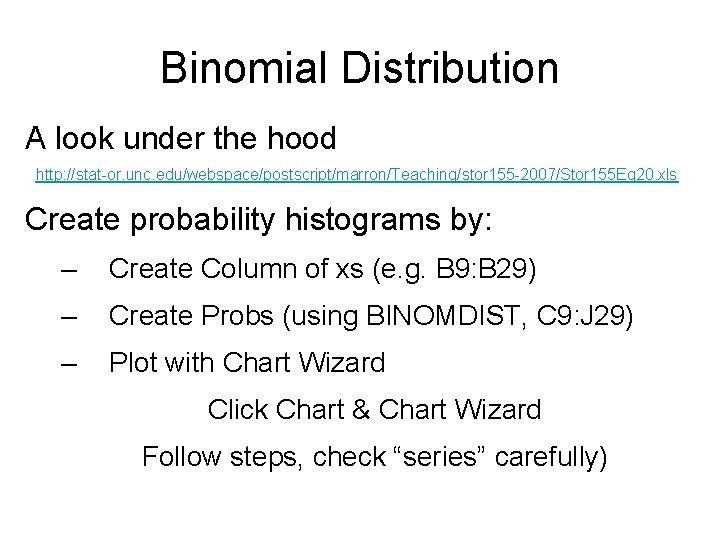
Binomial Distribution A look under the hood http: //stat-or. unc. edu/webspace/postscript/marron/Teaching/stor 155 -2007/Stor 155 Eg 20. xls Create probability histograms by: – Create Column of xs (e. g. B 9: B 29) – Create Probs (using BINOMDIST, C 9: J 29) – Plot with Chart Wizard Click Chart & Chart Wizard Follow steps, check “series” carefully)

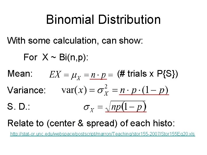
Binomial Distribution With some calculation, can show: For X ~ Bi(n, p): Mean: (# trials x P{S}) Variance: S. D. : Relate to (center & spread) of each histo: http: //stat-or. unc. edu/webspace/postscript/marron/Teaching/stor 155 -2007/Stor 155 Eg 20. xls

Binomial Distribution HW on Mean and Variance: 5. 5

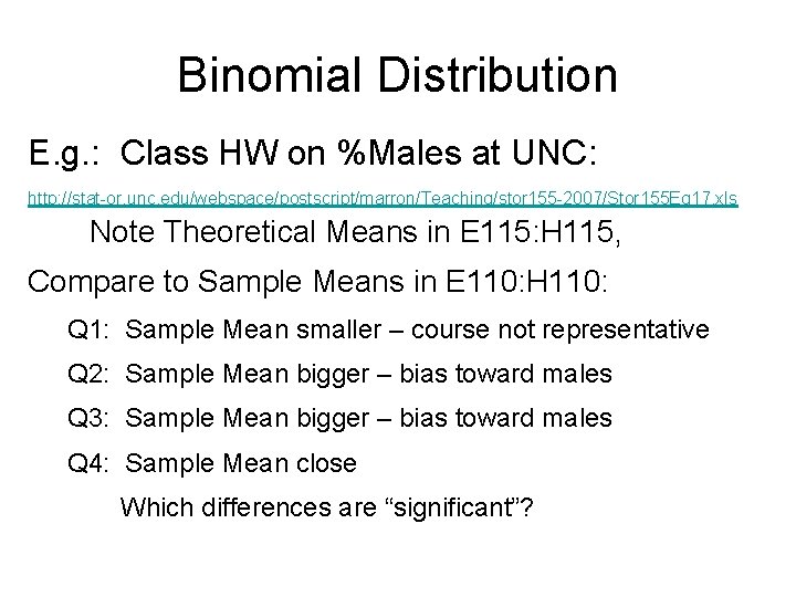
Binomial Distribution E. g. : Class HW on %Males at UNC: http: //stat-or. unc. edu/webspace/postscript/marron/Teaching/stor 155 -2007/Stor 155 Eg 17. xls Note Theoretical Means in E 115: H 115, Compare to Sample Means in E 110: H 110: Q 1: Sample Mean smaller – course not representative Q 2: Sample Mean bigger – bias toward males Q 3: Sample Mean bigger – bias toward males Q 4: Sample Mean close Which differences are “significant”?

Binomial Distribution E. g. : Class HW on %Males at UNC: http: //stat-or. unc. edu/webspace/postscript/marron/Teaching/stor 155 -2007/Stor 155 Eg 17. xls Note Theoretical SDs in E 116: H 115, 6 Compare to Sample SDs in E 112: H 112: Q 1: Sample SDs smaller – course population smaller Q 2: Sample SDs bigger – variety of doors (different p) Q 3: Sample SDs bigger – variety of choices (diff. p? ) Q 4: Sample SDs close Which differences are “significant”?

Binomial Distribution E. g. : Class HW on %Males at UNC: http: //stat-or. unc. edu/webspace/postscript/marron/Teaching/stor 155 -2007/Stor 155 Eg 17. xls Probability Histograms (see 3 rd column of plots), Good view of above ideas (for samples): Q 1: mean too small, not enough spread Q 2: mean too big, too spread Q 3: mean too big, too spread Q 4: looks “about right”…

Binomial Distribution HW: 5. 13 5. 19

And now for something completely different An Interesting and Relevant Issue: • “Places Rated” • Rankings Published by Several… • We’ve been #1? • Are we great ot what? Will take a careful look now

And now for something completely different Interesting Article: Analysis of Data from the Places Rated Almanac By: Richard A. Becker; Lorraine Denby; Robert Mc. Gill; Allan R. Wilks Published in: The American Statistician, Vol. 41, No. 3. (Aug. , 1987), pp. 169 -186. Hyperlink to JSTOR

And now for something completely different Main Ideas: • For data base used in ratings • Did careful analysis • In an unbiased way • Studied several aspects • An interesting issue: Who was “best”?

And now for something completely different Who was “best”? • Data base had 8 factors • How should we weight them? • Evenly? • Other choices? • Just choose some? (typical approach) • Can we make our city “best”?

And now for something completely different Who was “best”? • Approach: Consider all possible ratings (i. e. all sets of weights) • Which places can be #1? • Which places can be “worst”?

And now for something completely different Which places can be #1? • 134 cities are “best” • Including Raleigh Durham area Which places can be “worst”? • Even longer list here • But Raleigh Durham not here

And now for something completely different Which places can be #1? Which places can be “worst”? Interesting fact: Several cities on both lists!

And now for something completely different Some conclusions: • Be very skeptical of such ratings? • Ask: what happens if weights change? • Think: what motivates the rater? • Understand how other people can have different opinions (Just different “personal weights”)