Software Testing 1 Organization of this Lecture z

Software Testing 1

Organization of this Lecture z. Introduction to Testing. z. White-box testing: ystatement coverage ypath coverage ybranch testing ycondition coverage y. Cyclomatic complexity z. Summary 2

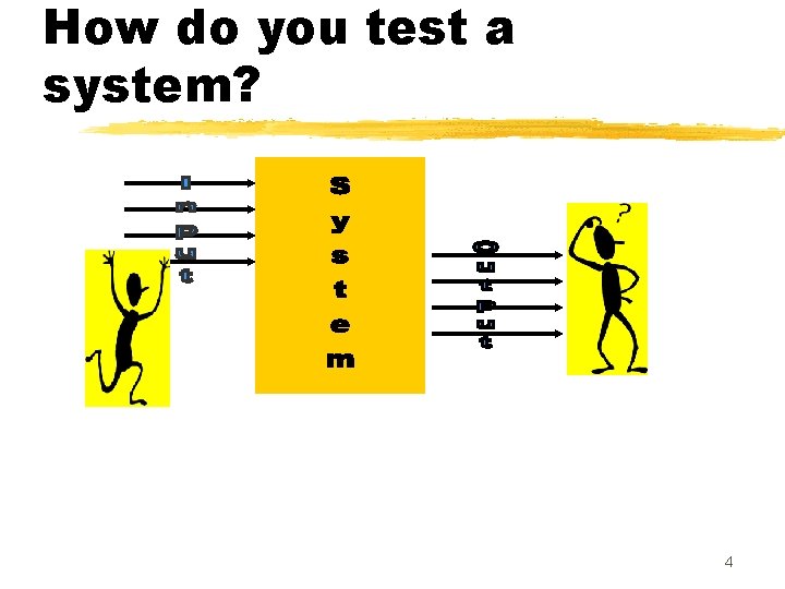
How do you test a system? z. Input test data to the system. z. Observe the output: y. Check if the system behaved as expected. 3

How do you test a system? 4

How do you test a system? z. If the program does not behave as expected: ynote the conditions under which it failed. ylater debug and correct. 5

Errors and Failures z. A failure is a manifestation of an error (aka defect or bug). ymere presence of an error may not lead to a failure. 6

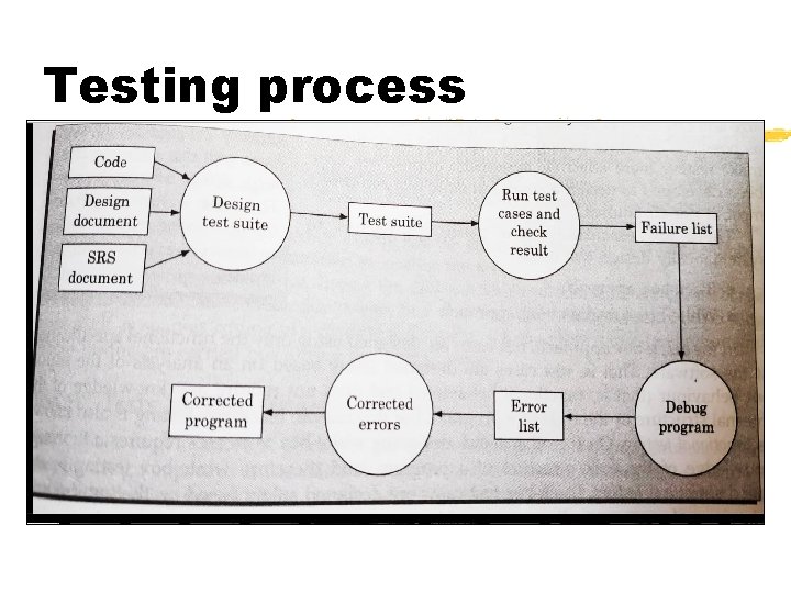
Test cases and Test suite z. Test a software using a set of carefully designed test cases: ythe set of all test cases is called the test suite 7

Test cases and Test suite z A test case is a triplet [I, S, O]: y. I is the data to be input to the system, y. S is the state of the system at which the data is input (like edit mode, view mode, create new or display data etc) y. O is the expected output from the system. 8

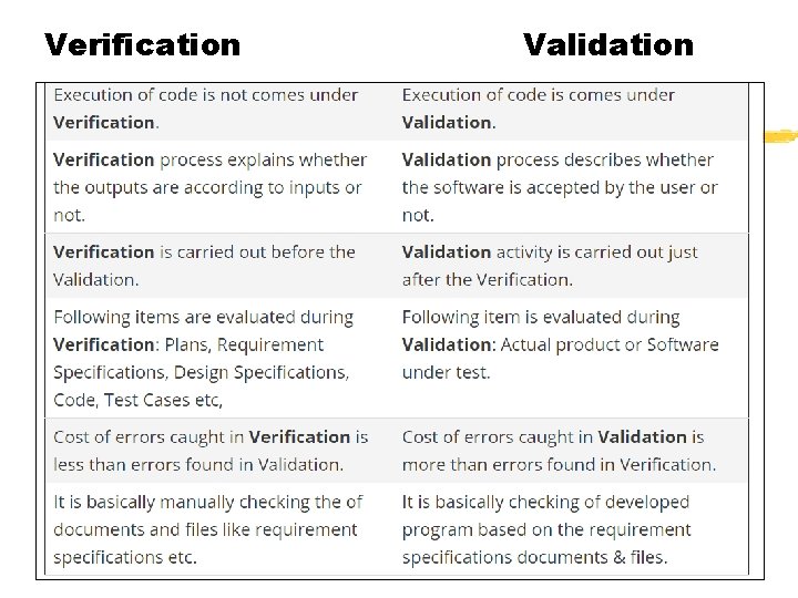
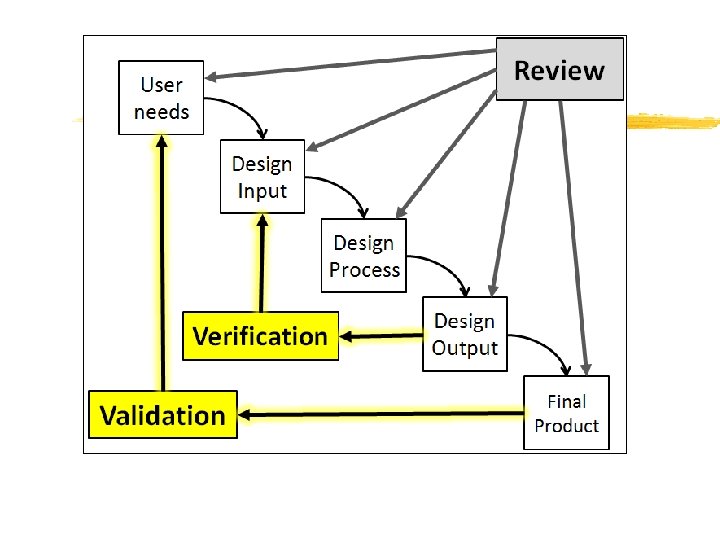
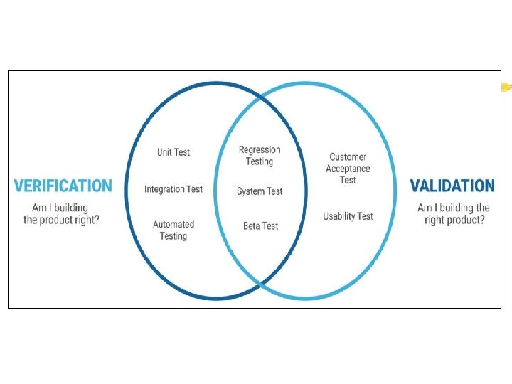
Verification versus Validation z. Verification is the process of determining: ywhether output of one phase of development conforms to its previous phase. z. Validation is the process of determining ywhether a fully developed system conforms to its SRS document. 9

Verification versus Validation z. Aim of Verification: yphase containment of errors z. Aim of validation: yfinal product is error free. 10

Verification versus Validation z. Verification: yare we doing right? z. Validation: yhave we done right? 11

Verification Validation

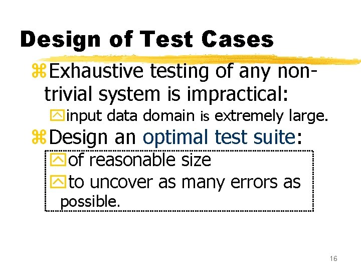
Design of Test Cases z. Exhaustive testing of any nontrivial system is impractical: yinput data domain is extremely large. z. Design an optimal test suite: yof reasonable size yto uncover as many errors as possible. 16

Design of Test Cases z. If test cases are selected randomly: ymany test cases do not contribute to the significance of the test suite, ydo not detect errors not already detected by other test cases in the suite. z. The number of test cases in a randomly selected test suite: ynot an indication of the effectiveness of the testing. 17

Design of Test Cases z. Testing a system using a large number of randomly selected test cases: ydoes not mean that many errors in the system will be uncovered. z. Consider an example: yfinding the maximum of two integers x and y. 18

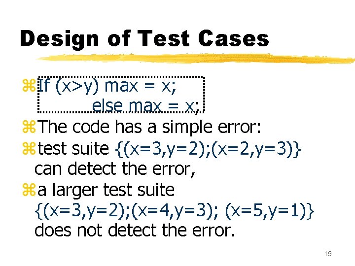
Design of Test Cases z. If (x>y) max = x; else max = x; z. The code has a simple error: ztest suite {(x=3, y=2); (x=2, y=3)} can detect the error, za larger test suite {(x=3, y=2); (x=4, y=3); (x=5, y=1)} does not detect the error. 19

Design of Test Cases z. Systematic approaches are required to design an optimal test suite: yeach test case in the suite should detect different errors. 20

Design of Test Cases z. Two main approaches to design test cases: y. Black-box approach y. White-box (or glass-box) approach 21

Testing process

Black-box Testing z. Test cases are designed using only functional specification of the software: ywithout any knowledge of the internal structure of the software. z. For this reason, black-box testing is also known as functional testing. 23

White-box Testing z. Designing white-box test cases: yrequires knowledge about the internal structure of software. ywhite-box testing is also called structural testing. 24

Black-box Testing z. Two main approaches to design black box test cases: y. Equivalence class partitioning y. Boundary value analysis 25

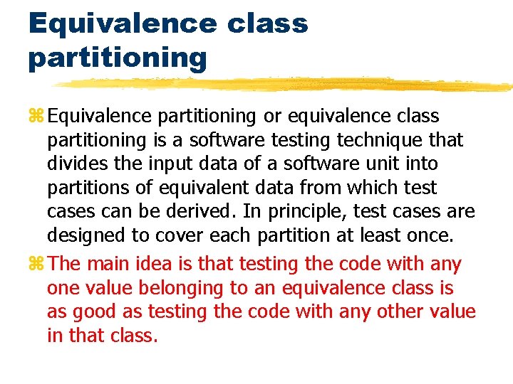
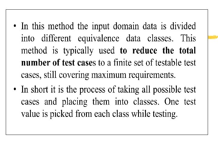
Equivalence class partitioning z Equivalence partitioning or equivalence class partitioning is a software testing technique that divides the input data of a software unit into partitions of equivalent data from which test cases can be derived. In principle, test cases are designed to cover each partition at least once. z The main idea is that testing the code with any one value belonging to an equivalence class is as good as testing the code with any other value in that class.

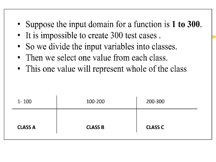
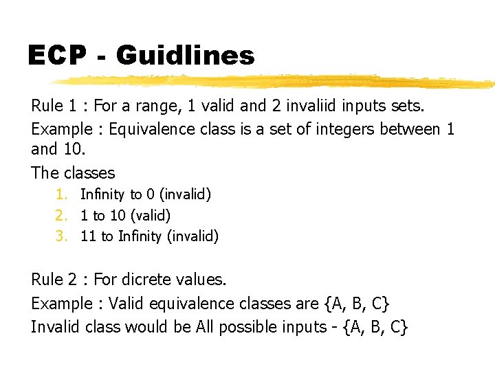
ECP - Guidlines Rule 1 : For a range, 1 valid and 2 invaliid inputs sets. Example : Equivalence class is a set of integers between 1 and 10. The classes 1. Infinity to 0 (invalid) 2. 1 to 10 (valid) 3. 11 to Infinity (invalid) Rule 2 : For dicrete values. Example : Valid equivalence classes are {A, B, C} Invalid class would be All possible inputs - {A, B, C}

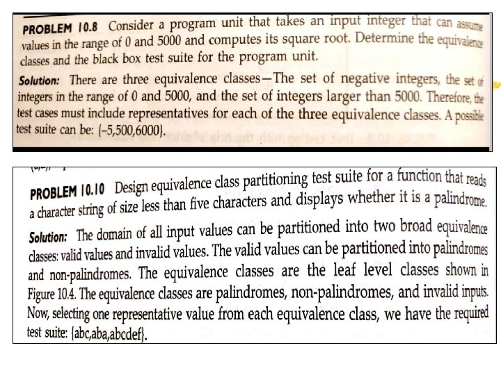
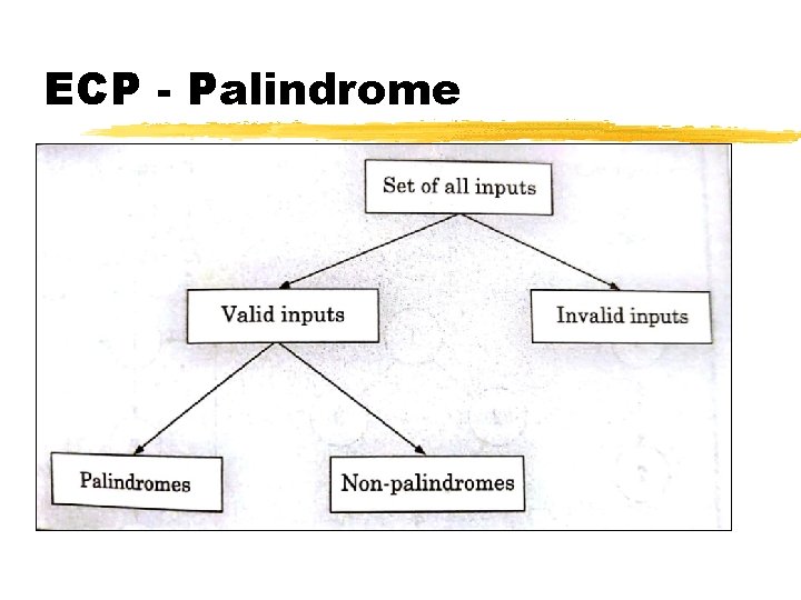
ECP - Palindrome

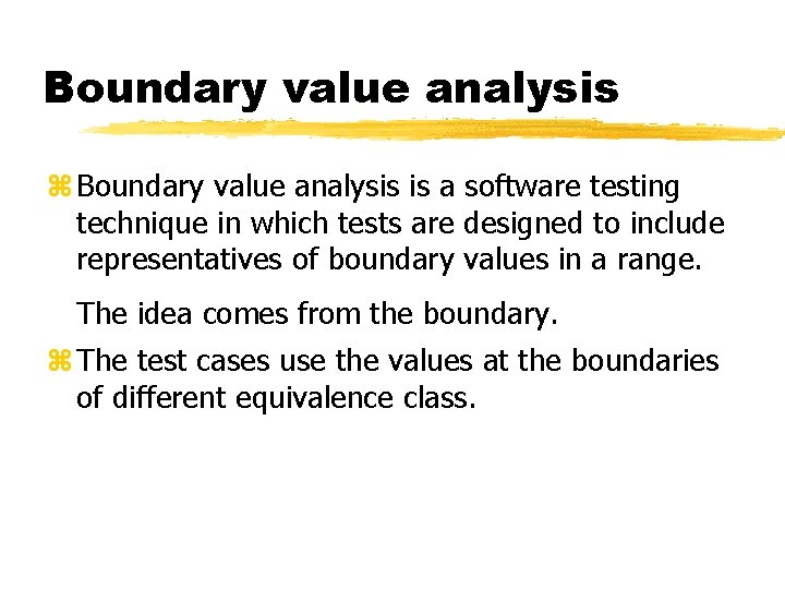
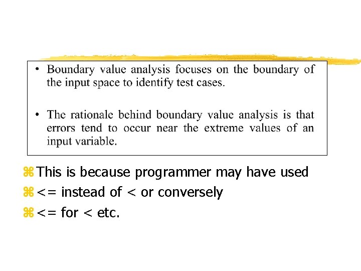
Boundary value analysis z Boundary value analysis is a software testing technique in which tests are designed to include representatives of boundary values in a range. The idea comes from the boundary. z The test cases use the values at the boundaries of different equivalence class.

z This is because programmer may have used z <= instead of < or conversely z <= for < etc.

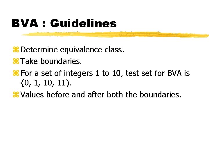
BVA : Guidelines z Determine equivalence class. z Take boundaries. z For a set of integers 1 to 10, test set for BVA is {0, 1, 10, 11). z Values before and after both the boundaries.

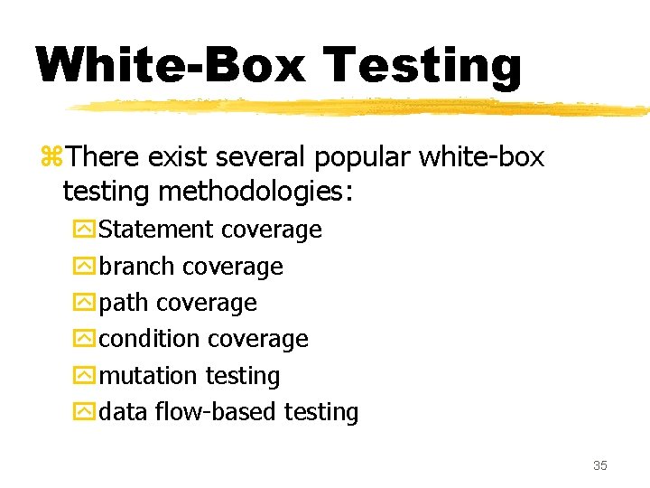
White-Box Testing z. There exist several popular white-box testing methodologies: y. Statement coverage ybranch coverage ypath coverage ycondition coverage ymutation testing ydata flow-based testing 35

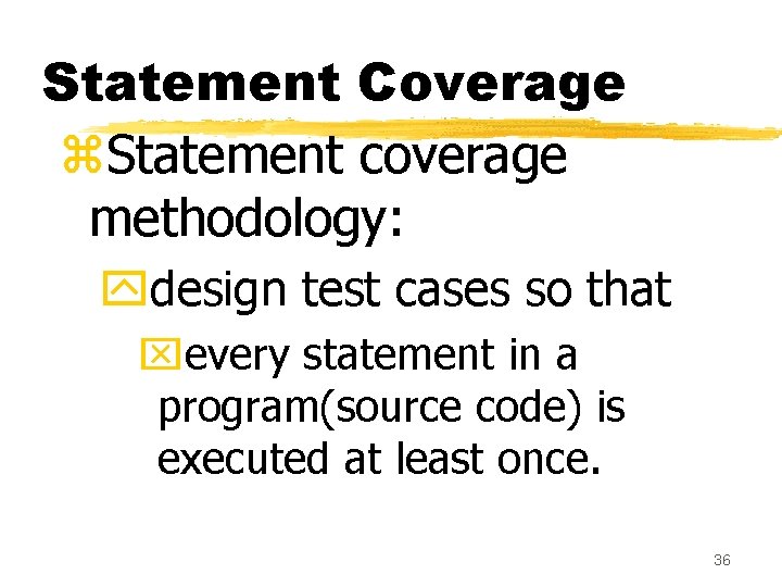
Statement Coverage z. Statement coverage methodology: ydesign test cases so that xevery statement in a program(source code) is executed at least once. 36

Statement Coverage z. The principal idea: yunless a statement is executed, ywe have no way of knowing if an error exists in that statement. 37

Statement coverage criterion z. Based on the observation: yan error in a program can not be discovered: xunless the part of the program containing the error is executed. 38

Statement coverage criterion z. Observing that a statement behaves properly for one input value: yno guarantee that it will behave correctly for all input values. 39

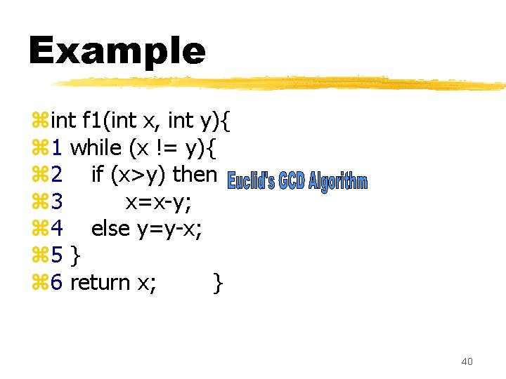
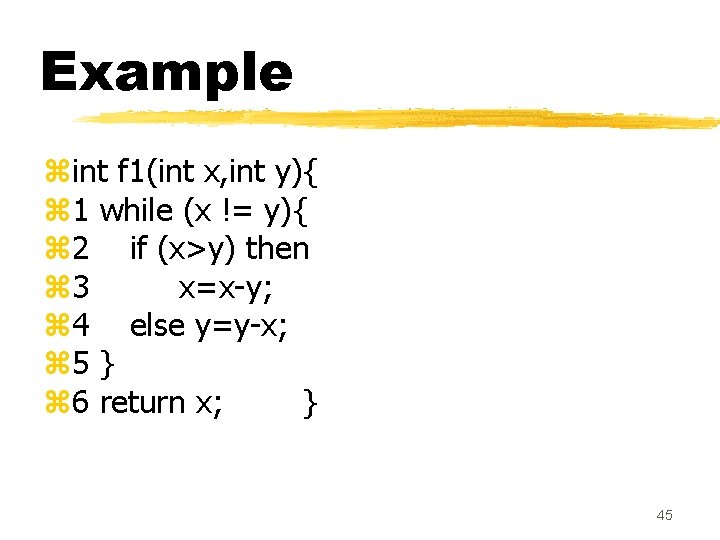
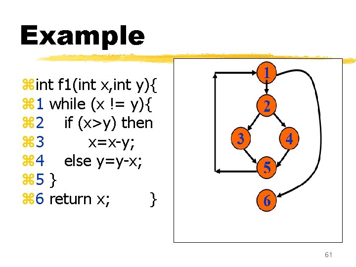
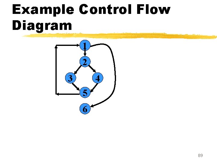
Example zint f 1(int x, int y){ z 1 while (x != y){ z 2 if (x>y) then z 3 x=x-y; z 4 else y=y-x; z 5 } z 6 return x; } 40

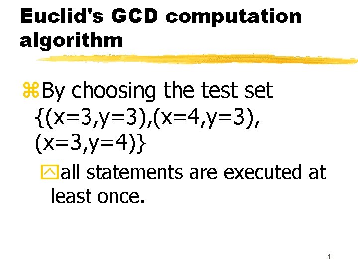
Euclid's GCD computation algorithm z. By choosing the test set {(x=3, y=3), (x=4, y=3), (x=3, y=4)} yall statements are executed at least once. 41

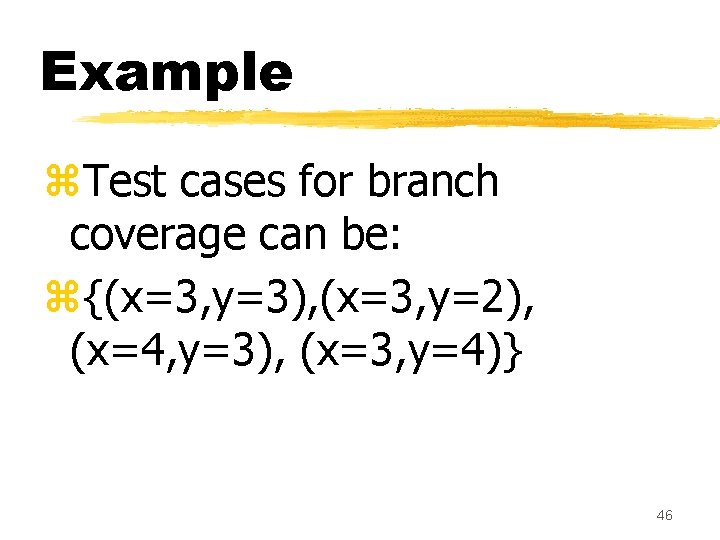
Branch Coverage z. Test cases are designed such that: ydifferent branch conditions xgiven true and false values in turn. 42

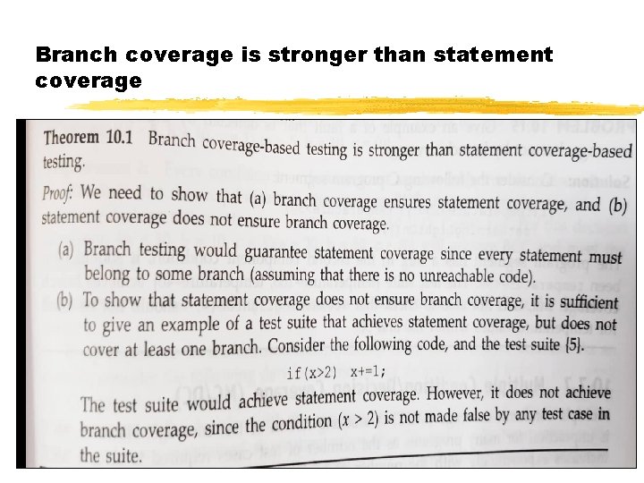
Branch Coverage z. Branch testing guarantees statement coverage: ya stronger testing compared to the statement coveragebased testing. 43

Stronger testing z. Test cases are a superset of a weaker testing: ydiscovers at least as many errors as a weaker testing ycontains at least as many significant test cases as a weaker test. 44

Example zint f 1(int x, int y){ z 1 while (x != y){ z 2 if (x>y) then z 3 x=x-y; z 4 else y=y-x; z 5 } z 6 return x; } 45

Example z. Test cases for branch coverage can be: z{(x=3, y=3), (x=3, y=2), (x=4, y=3), (x=3, y=4)} 46

Branch coverage is stronger than statement coverage

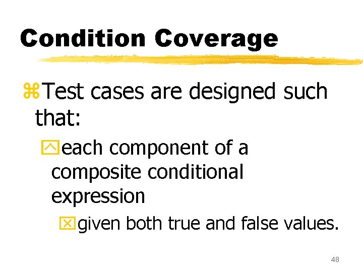
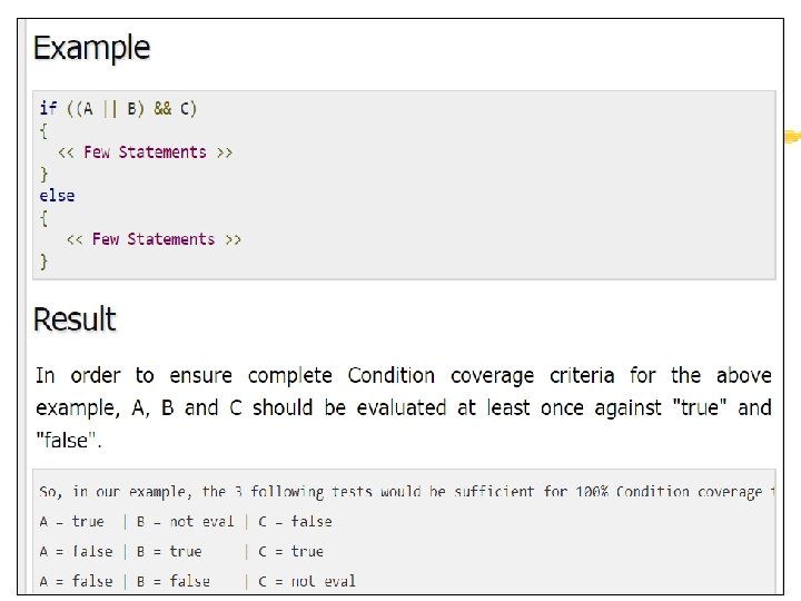
Condition Coverage z. Test cases are designed such that: yeach component of a composite conditional expression xgiven both true and false values. 48

z. C o n s i d e r Example t h e c o n 49

Branch testing z. Branch testing is the simplest condition testing strategy: ycompound conditions appearing in different branch statements xare given true and false values. 51

Comparision z. Condition testing (MCC) ystronger testing than branch testing: z. Branch testing ystronger than statement coverage testing. 52

Condition coverage z. Consider a boolean expression having n components: yfor condition coverage we n require 2 test cases. 53

Condition coverage z. Condition coverage-based testing technique: y practical only if n (the number of component conditions) is small. 54

Path Coverage z. Design test cases such that: yall linearly independent paths in the program are executed at least once. 55

Linearly independent paths z. Defined in terms of ycontrol flow graph (CFG) of a program. 56

Path coverage-based testing z. To understand the path coverage-based testing: ywe need to learn how to draw control flow graph of a program. 57

Control flow graph (CFG) z. A control flow graph (CFG) describes: ythe sequence in which different instructions of a program get executed. ythe way control flows through the program. 58

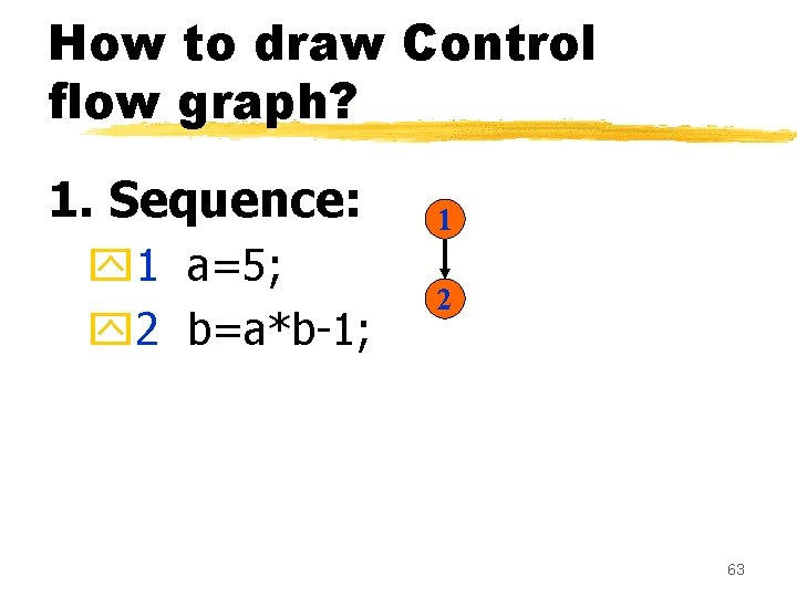
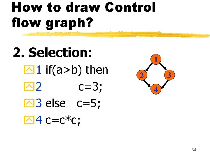
How to draw Control flow graph? z. Number all the statements of a program. z. Numbered statements: yrepresent nodes of the control flow graph. 59

How to draw Control flow graph? z. An edge from one node to another node exists: yif execution of the statement representing the first node xcan result in transfer of control to the other node. 60

Example zint f 1(int x, int y){ z 1 while (x != y){ z 2 if (x>y) then z 3 x=x-y; z 4 else y=y-x; z 5 } z 6 return x; } 61

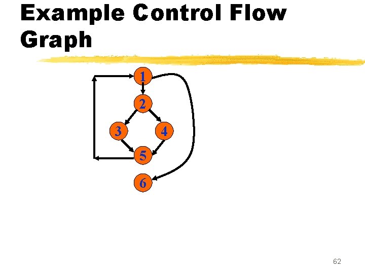
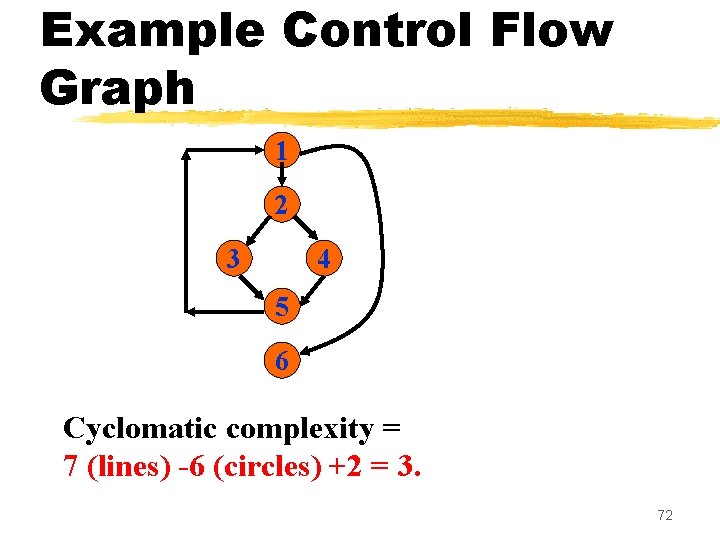
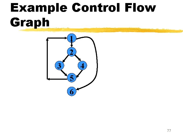
Example Control Flow Graph 1 2 3 4 5 6 62

How to draw Control flow graph? 1. Sequence: y 1 a=5; y 2 b=a*b-1; 1 2 63

How to draw Control flow graph? 2. Selection: y 1 if(a>b) then y 2 c=3; y 3 else c=5; y 4 c=c*c; 1 2 3 4 64

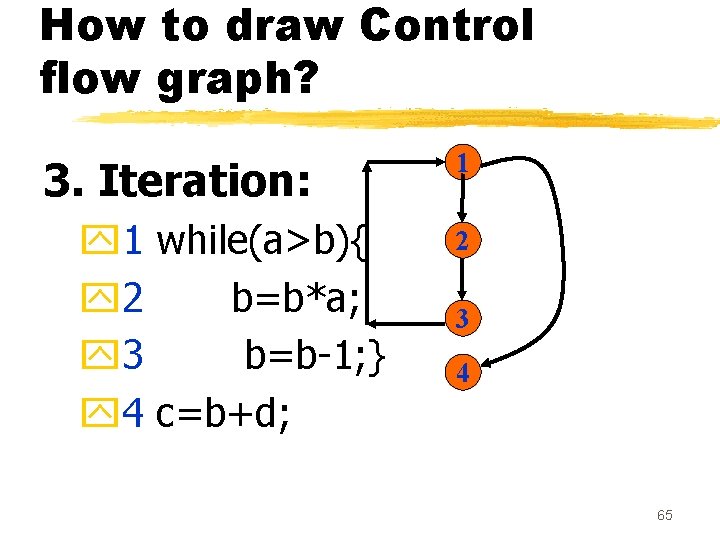
How to draw Control flow graph? 3. Iteration: y 1 while(a>b){ y 2 b=b*a; y 3 b=b-1; } y 4 c=b+d; 1 2 3 4 65

Path z. A path through a program: ya node and edge sequence from the starting node to a terminal node of the control flow graph. y There may be several terminal nodes for program. 66

Independent path z. Any path through the program: yintroducing at least one new node: xthat is not included in any other independent paths. 67

Independent path z. It is straight forward: yto identify linearly independent paths of simple programs. z. For complicated programs: yit is not so easy to determine the number of independent paths. 68

Mc. Cabe's cyclomatic metric z. An upper bound: yfor the number of linearly independent paths of a program z. Provides a practical way of determining: ythe maximum number of linearly independent paths in a program. 70

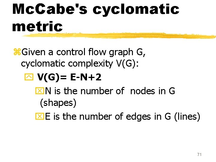
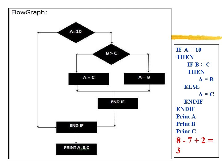
Mc. Cabe's cyclomatic metric z. Given a control flow graph G, cyclomatic complexity V(G): y V(G)= E-N+2 x. N is the number of nodes in G (shapes) x. E is the number of edges in G (lines) 71

Example Control Flow Graph 1 2 3 4 5 6 Cyclomatic complexity = 7 (lines) -6 (circles) +2 = 3. 72

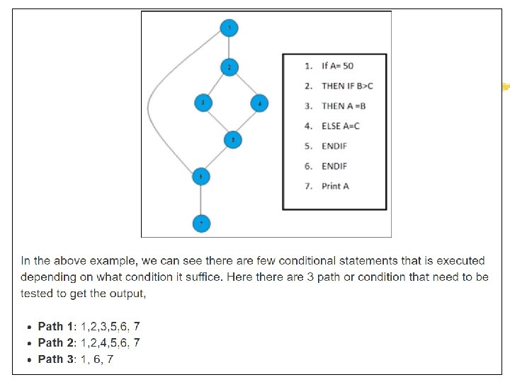
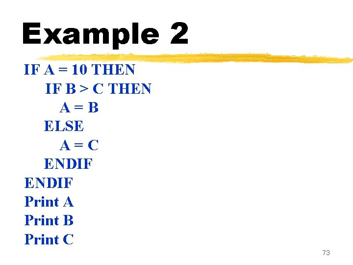
Example 2 IF A = 10 THEN IF B > C THEN A=B ELSE A=C ENDIF Print A Print B Print C 73

IF A = 10 THEN IF B > C THEN A=B ELSE A=C ENDIF Print A Print B Print C 8 -7+2= 3

Cyclomatic complexity z. Another way of computing cyclomatic complexity: yinspect control flow graph ydetermine number of bounded areas in the graph z. V(G) = Total number of bounded areas + 1 75

Bounded area z. Any region enclosed by a nodes and edge sequence. 76

Example Control Flow Graph 1 2 3 4 5 6 77

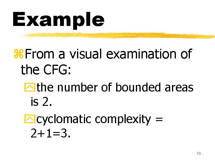
Example z. From a visual examination of the CFG: ythe number of bounded areas is 2. ycyclomatic complexity = 2+1=3. 78

Cyclomatic complexity z. Mc. Cabe's metric provides: xa quantitative measure of testing difficulty and the ultimate reliability z. Intuitively, ynumber of bounded areas increases with the number of decision nodes and loops. 79

Cyclomatic complexity z. The first method of computing V(G) is amenable to automation: yyou can write a program which determines the number of nodes and edges of a graph yapplies the formula to find V(G). 80

Cyclomatic complexity z. The cyclomatic complexity of a program provides: ya lower bound on the number of test cases to be designed yto guarantee coverage of all linearly independent paths. 81

Cyclomatic complexity z. Defines the number of independent paths in a program. z. Provides a lower bound: yfor the number of test cases for path coverage. 82

Cyclomatic complexity z. Knowing the number of test cases required: ydoes not make it any easier to derive the test cases, yonly gives an indication of the minimum number of test cases required. 83

Path testing z. The tester proposes: yan initial set of test data using his experience and judgement. 84

Path testing z. A dynamic program analyzer is used: yto indicate which parts of the program have been tested ythe output of the dynamic analysis xused to guide the tester in selecting additional test cases. 85

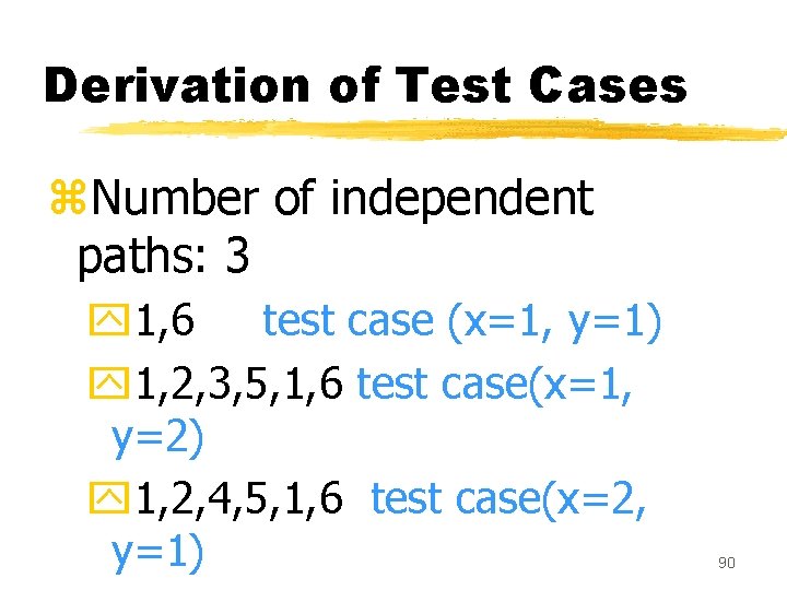
Derivation of Test Cases z. Let us discuss the steps: yto derive path coveragebased test cases of a program. 86

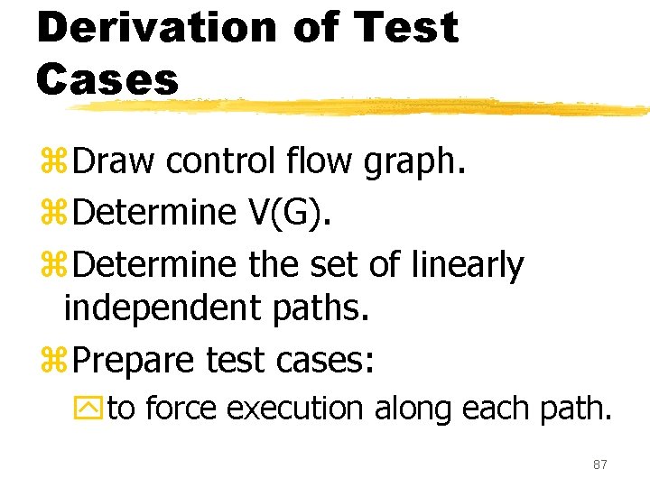
Derivation of Test Cases z. Draw control flow graph. z. Determine V(G). z. Determine the set of linearly independent paths. z. Prepare test cases: yto force execution along each path. 87

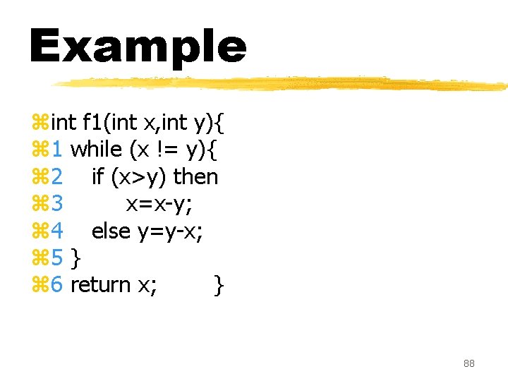
Example zint f 1(int x, int y){ z 1 while (x != y){ z 2 if (x>y) then z 3 x=x-y; z 4 else y=y-x; z 5 } z 6 return x; } 88

Example Control Flow Diagram 1 2 3 4 5 6 89

Derivation of Test Cases z. Number of independent paths: 3 y 1, 6 test case (x=1, y=1) y 1, 2, 3, 5, 1, 6 test case(x=1, y=2) y 1, 2, 4, 5, 1, 6 test case(x=2, y=1) 90

An interesting application of cyclomatic complexity z. Relationship exists between: y. Mc. Cabe's metric ythe number of errors existing in the code, ythe time required to find and correct the errors. 91

Cyclomatic complexity z. Cyclomatic complexity of a program: yalso indicates the psychological complexity of a program. ydifficulty level of understanding the program. 92

Cyclomatic complexity z. From maintenance perspective, ylimit cyclomatic complexity xof modules to some reasonable value. y. Good software development organizations: xrestrict cyclomatic complexity of functions to a maximum of ten or so. 93

Summary z. Exhaustive testing of nontrivial systems is impractical: ywe need to design an optimal set of test cases xshould expose as many errors as possible. 94

Summary z. If we select test cases randomly: ymany of the selected test cases do not add to the significance of the test set. 95

Summary z. There are two approaches to testing: yblack-box testing and ywhite-box testing. 96

Summary z. Designing test cases for black box testing: ydoes not require any knowledge of how the functions have been designed and implemented. y. Test cases can be designed by examining only SRS document. 97

Summary z. White box testing: yrequires knowledge about internals of the software. y. Design and code is required. 98

Summary z. We have discussed a few whitebox test strategies. y. Statement coverage ybranch coverage ycondition coverage ypath coverage 99

Summary z. A stronger testing strategy: yprovides more number of significant test cases than a weaker one. y. Condition coverage is strongest among strategies we discussed. 100

Summary z. We discussed Mc. Cabe’s Cyclomatic complexity metric: yprovides an upper bound for linearly independent paths ycorrelates with understanding, testing, and debugging difficulty of a program. 101