Simulating and Modeling Genetically Informative Data Matthew C

Simulating and Modeling Genetically Informative Data Matthew C. Keller Sarah E. Medland

Outline n n n The usefulness of simulation in behavioral genetics Using Gene. Evolve to simulate genetically informative data Practical simulating different designs 1. 2. Classical Twin Design (CTD) Nuclear Twin Family Design (NTFD)

Simulation provides knowledge about processes that are difficult/impossible to figure out analytically n Independent check of models. Especially important for complex (e. g. , extended twin family) models. Ø Ø n Model verification: Check that your models work as they are supposed to. Sensitivity analysis: Check the effect on parameter estimates when assumptions are violated (e. g. , different modes of assortative mating, vertical transmission, or genetic action). Method for predicting complex dynamics in population genetics

Using complex models without independent verification (e. g. , simulation) is like…

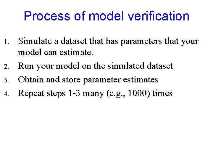
Process of model verification 1. 2. 3. 4. Simulate a dataset that has parameters that your model can estimate. Run your model on the simulated dataset Obtain and store parameter estimates Repeat steps 1 -3 many (e. g. , 1000) times

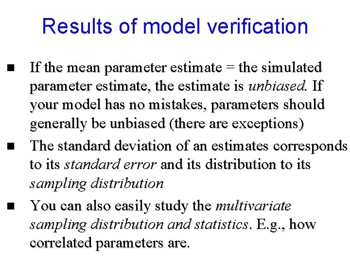
Results of model verification n If the mean parameter estimate = the simulated parameter estimate, the estimate is unbiased. If your model has no mistakes, parameters should generally be unbiased (there are exceptions) The standard deviation of an estimates corresponds to its standard error and its distribution to its sampling distribution You can also easily study the multivariate sampling distribution and statistics. E. g. , how correlated parameters are.

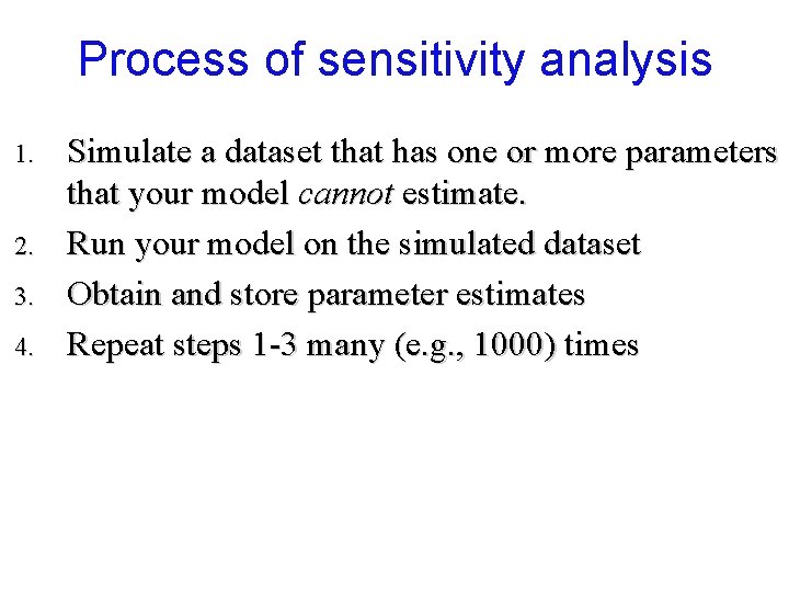
Process of sensitivity analysis 1. 2. 3. 4. Simulate a dataset that has one or more parameters that your model cannot estimate. Run your model on the simulated dataset Obtain and store parameter estimates Repeat steps 1 -3 many (e. g. , 1000) times

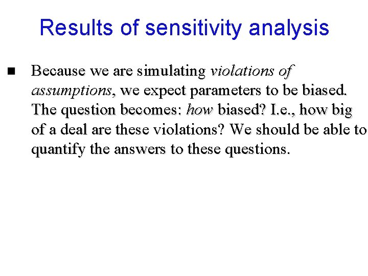
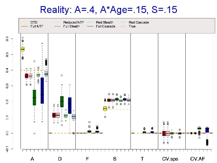
Results of sensitivity analysis n Because we are simulating violations of assumptions, we expect parameters to be biased. The question becomes: how biased? I. e. , how big of a deal are these violations? We should be able to quantify the answers to these questions.

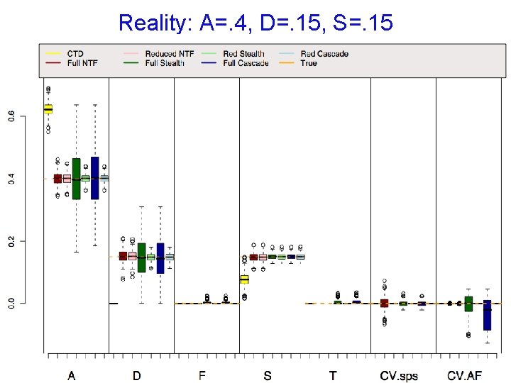
Reality: A=. 4, D=. 15, S=. 15

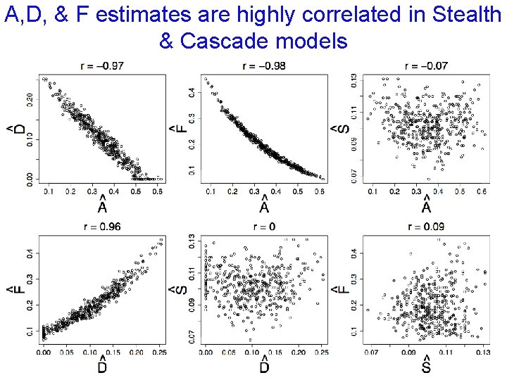
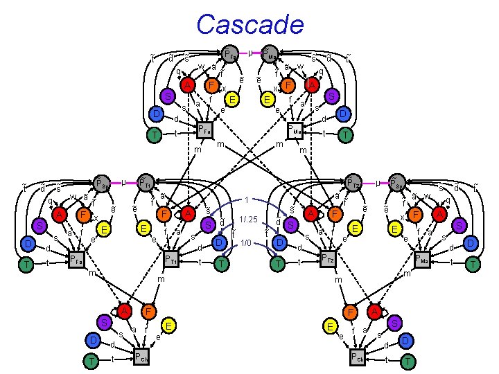
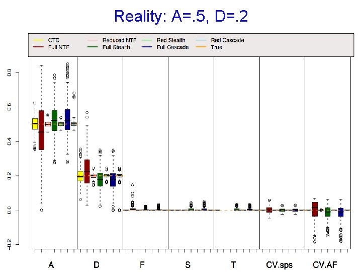
A, D, & F estimates are highly correlated in Stealth & Cascade models

Simulation is not a panacea n n Simulation can be said to provide “knowledge without understanding. ” It is a helpful tool for understanding, but doesn’t provide understanding in and of itself. Simulations themselves rely on assumptions about how processes work. If these are wrong, our simulation results may not reflect reality.

Simulation program: Gene. Evolve

Gene. Evolve 0. 73 n Implemented in R, open-source, user modifiable User specifies 31 basic parameters up front (and 17 advanced ones); no need to alter script after that. n Fast (on AMD Opteron 3. 2 GHz dual 64 bit processor, 2 GB RAM; OS= RHEL AS 4) n u 10 genes, N=20, 000 takes ~ 20 seconds/gen Download: www. matthewckeller. com

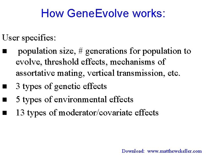
How Gene. Evolve works: User specifies: n population size, # generations for population to evolve, threshold effects, mechanisms of assortative mating, vertical transmission, etc. n 3 types of genetic effects n 5 types of environmental effects n 13 types of moderator/covariate effects Download: www. matthewckeller. com

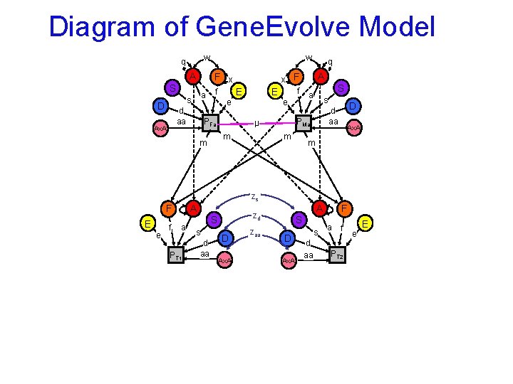
Diagram of Gene. Evolve Model w q A F x S a s D d aa Ax. A w f e PFa x F f E e E A S a s m D d aa PMa µ m m q Ax. A m zs A F E e f a PT 1 S s d aa A zd D Ax. A zaa S D Ax. A s d aa F a f PT 2 e E

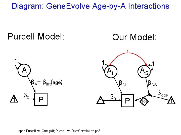
Diagram: Gene. Evolve Age-by-A Interactions Purcell Model: Our Model: r 1 1 A βA+ βint(age) 1 β 0 AS AL P βAL 1 open Purcell-vs-Ours. pdf; Purcell-vs-Ours. Correlation. pdf β 0 P 1 βAS βage 1

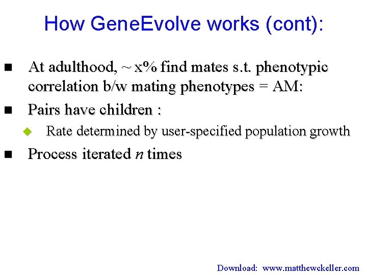
How Gene. Evolve works (cont): n n At adulthood, ~ x% find mates s. t. phenotypic correlation b/w mating phenotypes = AM: Pairs have children : u n Rate determined by user-specified population growth Process iterated n times Download: www. matthewckeller. com

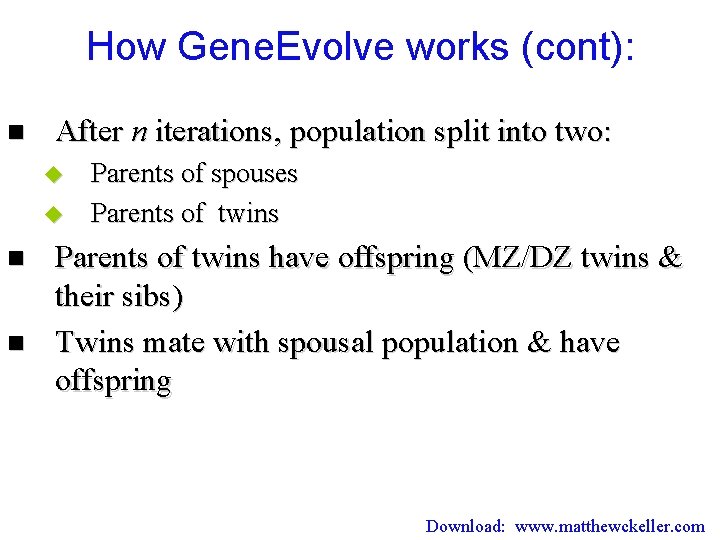
How Gene. Evolve works (cont): n After n iterations, population split into two: u u n n Parents of spouses Parents of twins have offspring (MZ/DZ twins & their sibs) Twins mate with spousal population & have offspring Download: www. matthewckeller. com

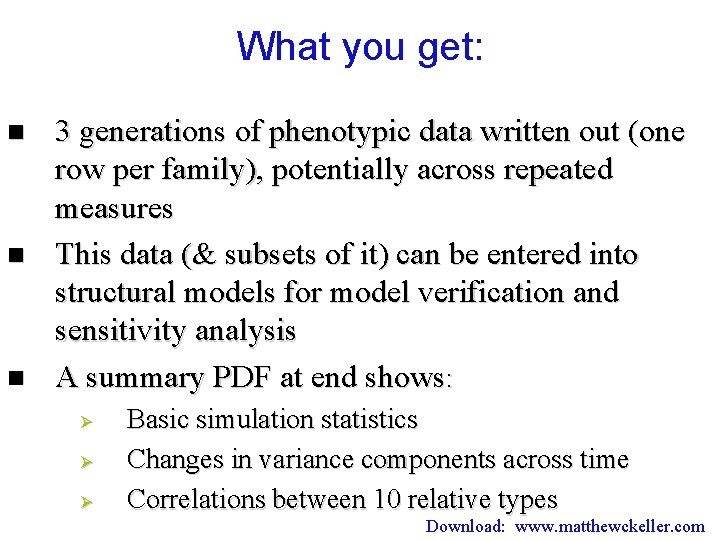
What you get: n n n 3 generations of phenotypic data written out (one row per family), potentially across repeated measures This data (& subsets of it) can be entered into structural models for model verification and sensitivity analysis A summary PDF at end shows: Ø Ø Ø Basic simulation statistics Changes in variance components across time Correlations between 10 relative types Download: www. matthewckeller. com

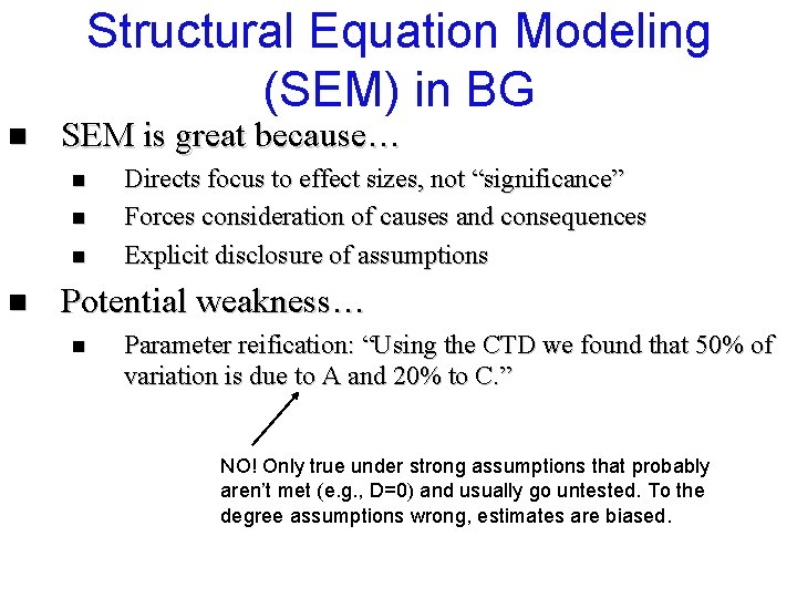
Structural Equation Modeling (SEM) in BG n SEM is great because… n n Directs focus to effect sizes, not “significance” Forces consideration of causes and consequences Explicit disclosure of assumptions Potential weakness… n Parameter reification: “Using the CTD we found that 50% of variation is due to A and 20% to C. ”

Structural Equation Modeling (SEM) in BG n SEM is great because… n n Directs focus to effect sizes, not “significance” Forces consideration of causes and consequences Explicit disclosure of assumptions Potential weakness… n Parameter reification: “Using the CTD we found that 50% of variation is due to A and 20% to C. ” NO! Only true under strong assumptions that probably aren’t met (e. g. , D=0) and usually go untested. To the degree assumptions wrong, estimates are biased.

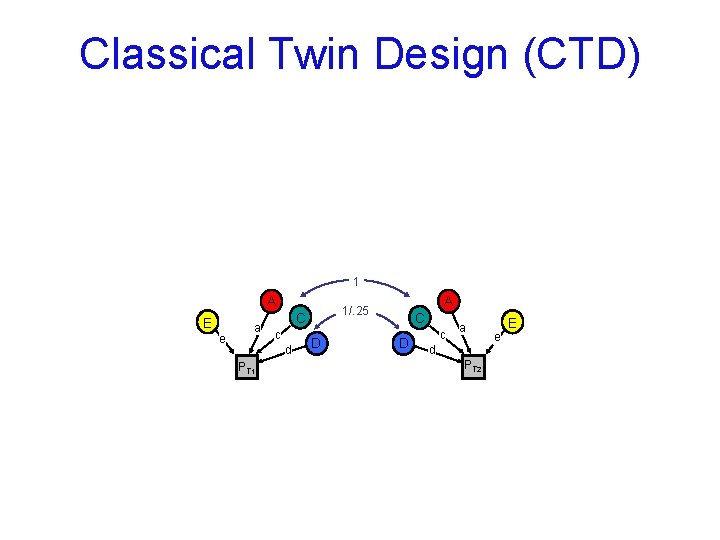
Classical Twin Design (CTD) 1 A E e a C c d PT 1 A 1/. 25 D C D c a d PT 2 e E

Classical Twin Design (CTD) n Assumption biased up Either D or C is zero No assortative mating No A-C covariance biased down A C C C&D D D&A 1 A E e a C c d PT 1 A 1/. 25 D C D c a d PT 2 e E

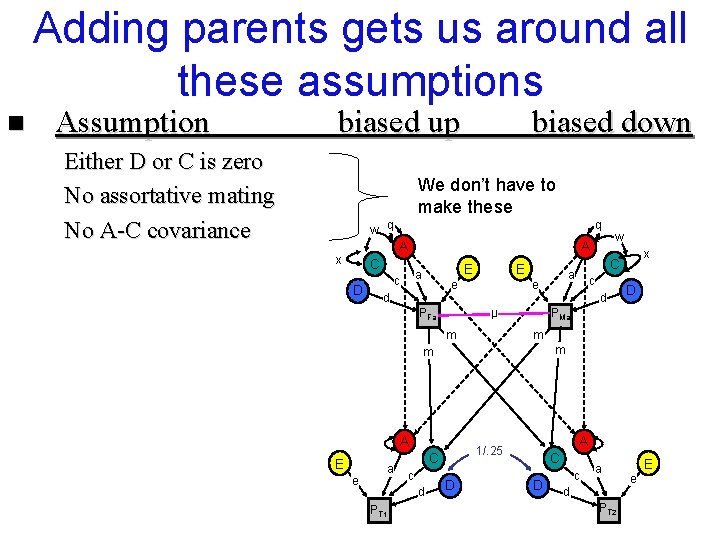
Adding parents gets us around all these assumptions n Assumption biased up Either D or C is zero No assortative mating No A-C covariance biased down We don’t have to make these w q q A x C D A E a c E e d PFa µ m e d PT 1 D m A 1/. 25 C c d m A a c PMa m E x C a e w D C D c a d PT 2 E e

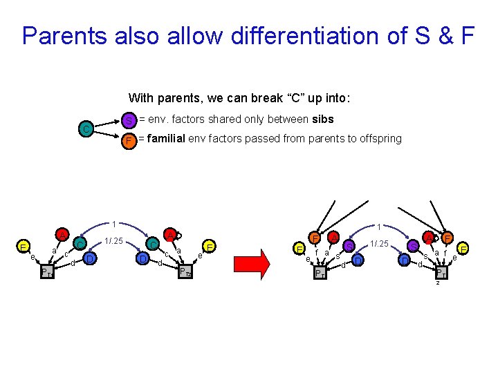
Parents also allow differentiation of S & F With parents, we can break “C” up into: SS = env. factors shared only between sibs C FF = familial env factors passed from parents to offspring 1 A E e a c PT 1 1/. 25 C d D C D 1 A d c a PT 2 e E F E e A f a s PT 1 1/. 25 S d D S D d A F E s a f e PT 2

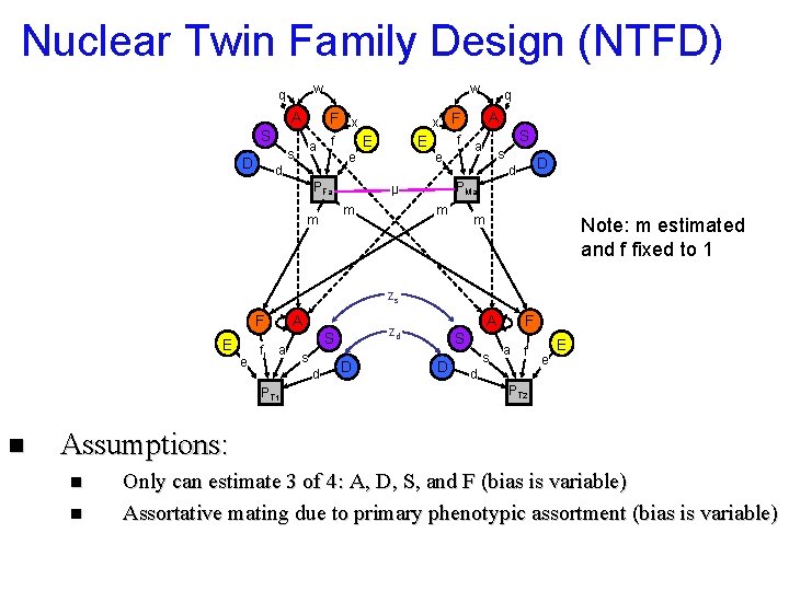
Nuclear Twin Family Design (NTFD) w q A F x S a s D w f e d PFa x F f E e E A S a s D d PMa µ m m q m m Note: m estimated and f fixed to 1 zs A F E e f a d PT 1 n S s A zd D S D s F a f d e E PT 2 Assumptions: n n Only can estimate 3 of 4: A, D, S, and F (bias is variable) Assortative mating due to primary phenotypic assortment (bias is variable)

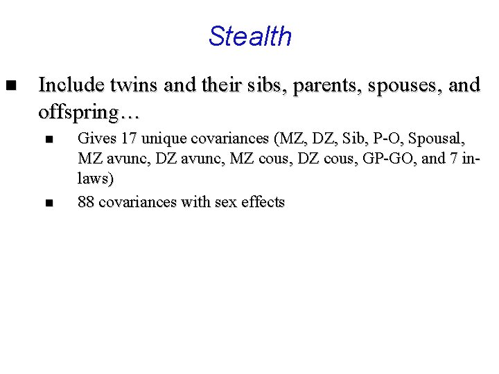
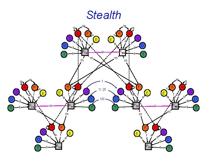
Stealth n Include twins and their sibs, parents, spouses, and offspring… n n Gives 17 unique covariances (MZ, DZ, Sib, P-O, Spousal, MZ avunc, DZ avunc, MZ cous, DZ cous, GP-GO, and 7 inlaws) 88 covariances with sex effects

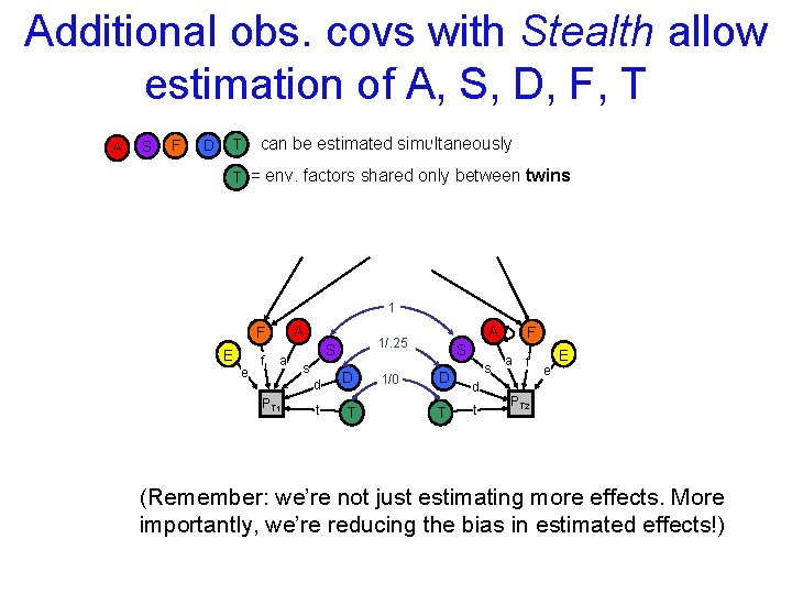
Additional obs. covs with Stealth allow estimation of A, S, D, F, T A S F D T can be estimated simultaneously T = env. factors shared only between twins 1 A F E e f a S s d PT 1 t A 1/. 25 D T 1/0 S D T s d t F a f e E PT 2 (Remember: we’re not just estimating more effects. More importantly, we’re reducing the bias in estimated effects!)

Stealth w q A F x S a s D w f e d PFa t T S D T s f e E E f e S a s m D d PMa t T m w PT 1 m s t D T 1/0 S D T s F S s e d t a f PCh E E PT 2 m A F e E e f a S s d PCh f a t D T q A S s d PMa m E e µ F d t x F a f m A T a A 1/. 25 S d µ PFa D A F F x a A 1 d t µ w A E m m q x F f E e q t D T

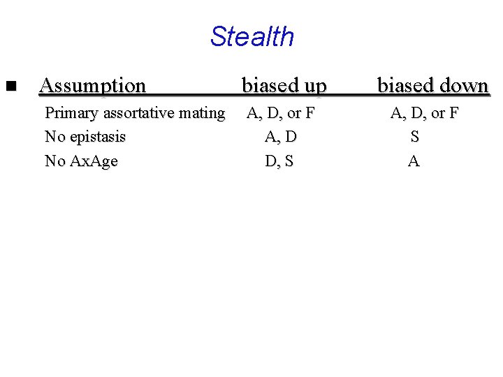
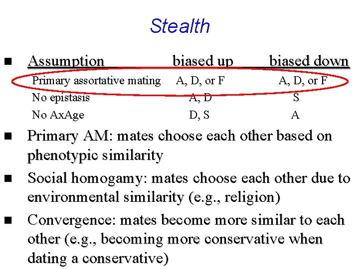
Stealth n Assumption Primary assortative mating No epistasis No Ax. Age biased up A, D, or F A, D D, S biased down A, D, or F S A

Stealth n Assumption Primary assortative mating No epistasis No Ax. Age n n n biased up A, D, or F A, D D, S biased down A, D, or F S A Primary AM: mates choose each other based on phenotypic similarity Social homogamy: mates choose each other due to environmental similarity (e. g. , religion) Convergence: mates become more similar to each other (e. g. , becoming more conservative when dating a conservative)

Cascade ~ d ~ t ~ PFa ~ s w ~ a ~ f q A S a s D f e d ~ s q ~ PSp w ~ a ~ f A S D T s F x a f d t e E f e a m S a s D d t T m s t D T ~ s 1/. 25 ~ t 1/0 ~ a ~ f ~t A ~ d S D T s a f S s d t a f PCh ~ e E x F E m m E e E f a A e f a S s d PCh t D T ~ s ~ d ~ t q A S s d PMa F e ~ ~ a w f PT 2 F d t e ~ PSp µ ~ e F m A T ~ S d d PT 1 1 ~s A F PFa D A ~ PT 2 ~ ~ a f ~ e E ~ t q PMa m ~ d ~ PT 1 µ ~ e E x F f E e m m ~ t ~ e ~ s ~ ~ a w f PFa t T ~ e F x ~ PMa µ t D T

Reality: A=. 5, D=. 2

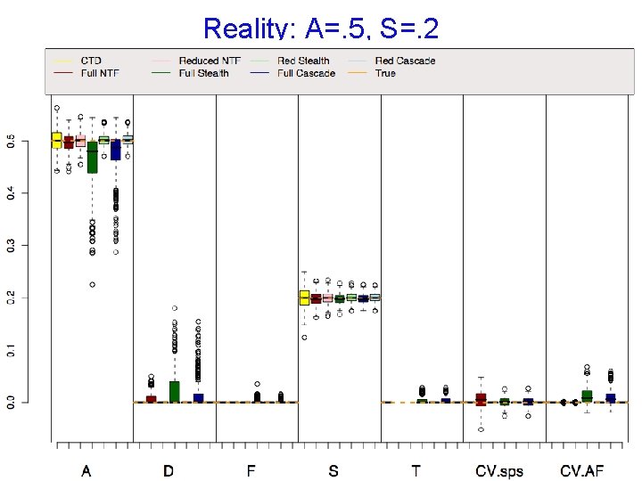
Reality: A=. 5, S=. 2

Reality: A=. 4, D=. 15, S=. 15

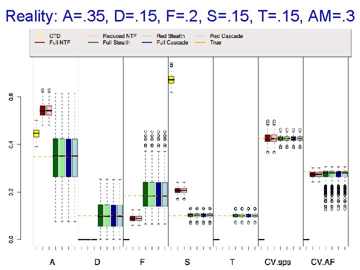
Reality: A=. 35, D=. 15, F=. 2, S=. 15, T=. 15, AM=. 3

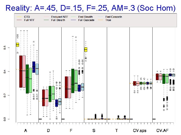
Reality: A=. 45, D=. 15, F=. 25, AM=. 3 (Soc Hom)

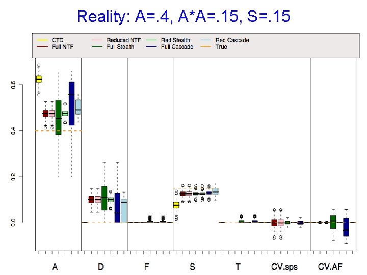
Reality: A=. 4, A*A=. 15, S=. 15

Reality: A=. 4, A*Age=. 15, S=. 15

Conclusions n n All models require assumptions. Generally, more assumptions = more biased estimates For the first time, we have demonstrated independent assessments of the NTFD, Stealth, and Cascade models n These complicated models work as designed! n In all models, but especially the CTD, please don’t REIFY A, C, & D!

Acknowledgments n n Those who conceived of these models originally: n Jinks, Fulker, Eaves, Cloninger, Reich, Rice, Heath, Neale, Maes, etc. And to Nick Martin: for his energy and enthusiasm, and for encouraging us to do this to begin with

Why use it? Modeling aid n Check bias & identification: u n Check model’s sensitivity to assumptions: u n Feed PE parameters you are modeling, simulate data, & see if your model recovers the parameters Simulate violations of assumptions & note its effects on estimates Estimate power & multivariate sampling dist’s of estimates under very general conditions: u Run PE multiple times given whatever condition you want Download: www. matthewckeller. com

Why use it? Predictor of population / evolutionary genetics dynamics n n n Find changes in variance parameters & relative covariances under different modes of AM, VT, & genetic effects: Simulate random genetic drift by varying population size Introduce selection (coming) to test theories on maintenance of genetic variation Download: www. matthewckeller. com