Simple Regression Social Research Methods 2109 6507 Spring

Simple Regression (簡單迴歸分析) Social Research Methods 2109 & 6507 Spring, 2006 March 8, 9, 13, 2006 1

From Correlation to Regression: • Correlation (相關分析、相關係數): measures the strength of linear association between 2 quantitative variables (二變數線性關係的強度) • Regression (迴歸分析): 1. Description (描述): summarize the relationship between the two variables with a straight line, what does the line look like? (如何用一直線描 述二變數的關係? ) 2. Prediction (預測): how to make predictions about one variable based on another? (如何從 一變數預測另一變數? ) 2

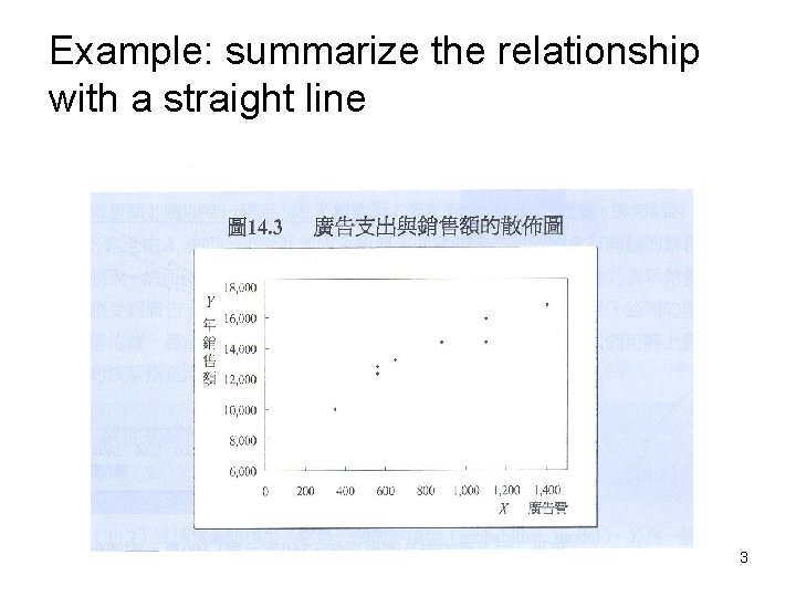
Example: summarize the relationship with a straight line 3

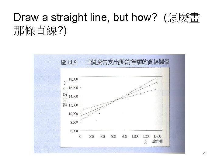
Draw a straight line, but how? (怎麼畫 那條直線? ) 4

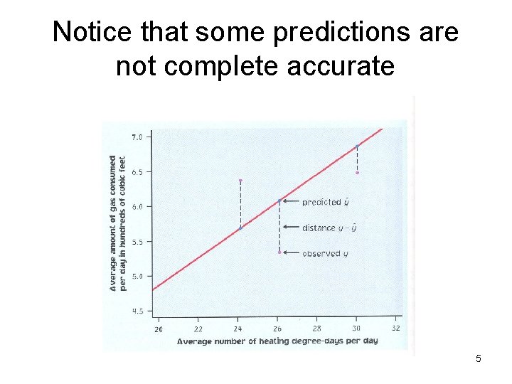
Notice that some predictions are not complete accurate 5

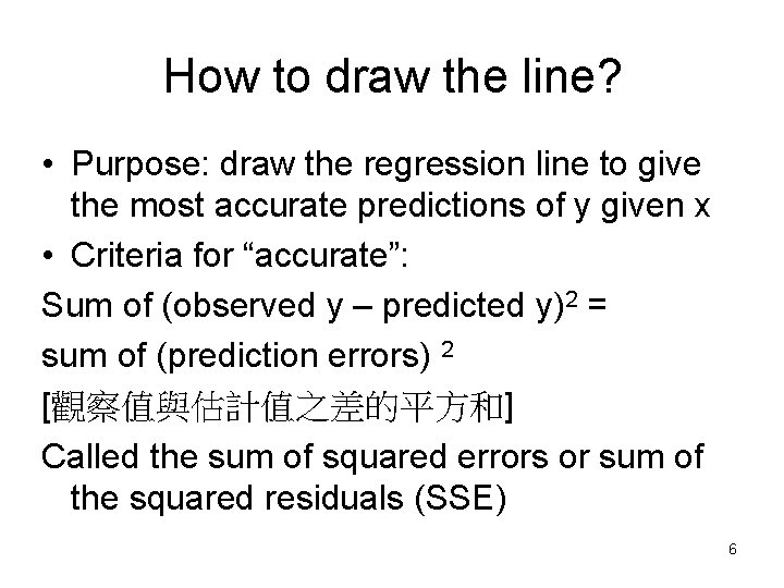
How to draw the line? • Purpose: draw the regression line to give the most accurate predictions of y given x • Criteria for “accurate”: Sum of (observed y – predicted y)2 = sum of (prediction errors) 2 [觀察值與估計值之差的平方和] Called the sum of squared errors or sum of the squared residuals (SSE) 6

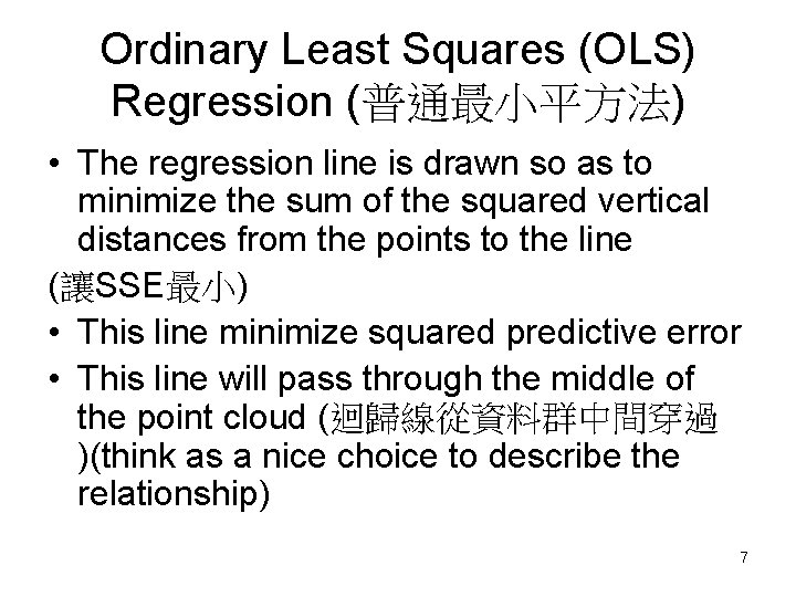
Ordinary Least Squares (OLS) Regression (普通最小平方法) • The regression line is drawn so as to minimize the sum of the squared vertical distances from the points to the line (讓SSE最小) • This line minimize squared predictive error • This line will pass through the middle of the point cloud (迴歸線從資料群中間穿過 )(think as a nice choice to describe the relationship) 7

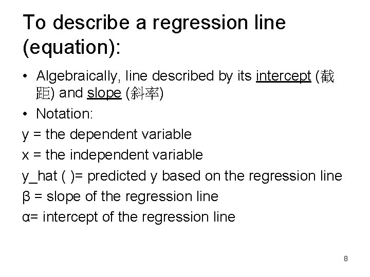
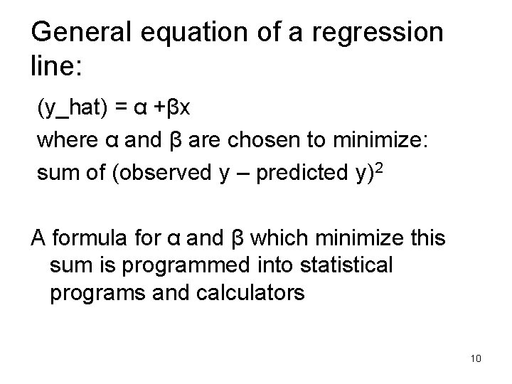
To describe a regression line (equation): • Algebraically, line described by its intercept (截 距) and slope (斜率) • Notation: y = the dependent variable x = the independent variable y_hat ( )= predicted y based on the regression line β = slope of the regression line α= intercept of the regression line 8

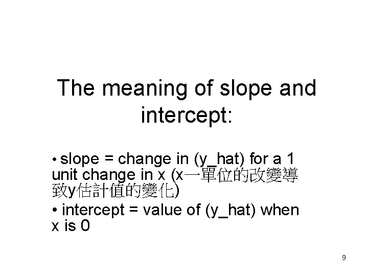
The meaning of slope and intercept: • slope = change in (y_hat) for a 1 unit change in x (x一單位的改變導 致y估計值的變化) • intercept = value of (y_hat) when x is 0 9

General equation of a regression line: (y_hat) = α +βx where α and β are chosen to minimize: sum of (observed y – predicted y)2 A formula for α and β which minimize this sum is programmed into statistical programs and calculators 10

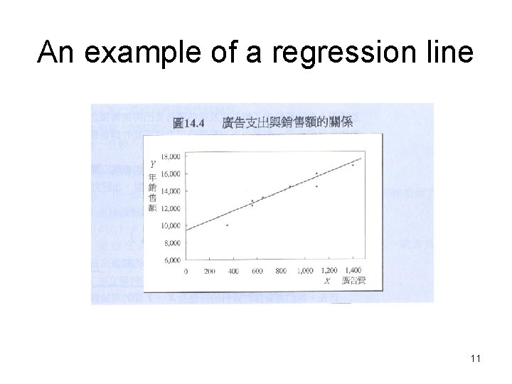
An example of a regression line 11

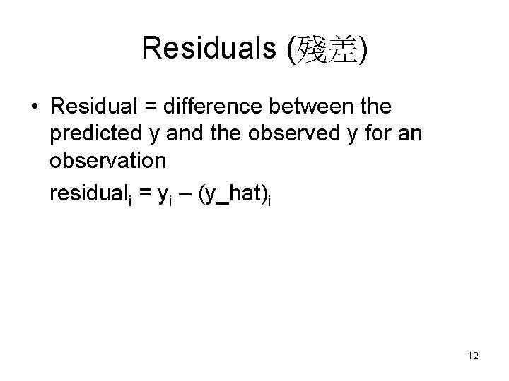
Residuals (殘差) • Residual = difference between the predicted y and the observed y for an observation residuali = yi – (y_hat)i 12

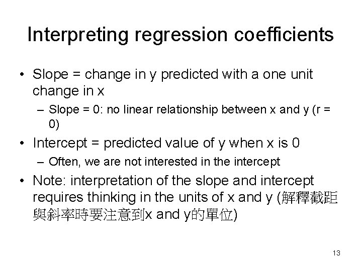
Interpreting regression coefficients • Slope = change in y predicted with a one unit change in x – Slope = 0: no linear relationship between x and y (r = 0) • Intercept = predicted value of y when x is 0 – Often, we are not interested in the intercept • Note: interpretation of the slope and intercept requires thinking in the units of x and y (解釋截距 與斜率時要注意到x and y的單位) 13

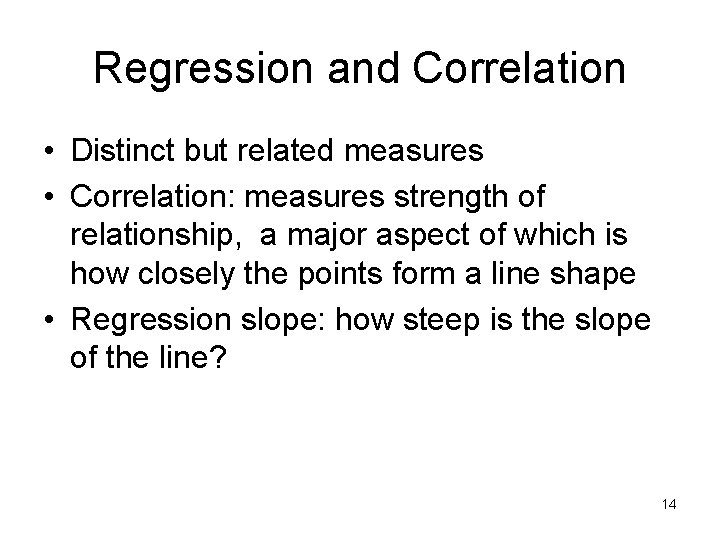
Regression and Correlation • Distinct but related measures • Correlation: measures strength of relationship, a major aspect of which is how closely the points form a line shape • Regression slope: how steep is the slope of the line? 14

To get slope and intercept for a regression: 15

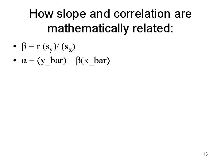
How slope and correlation are mathematically related: • β = r (sy)/ (sx) • α = (y_bar) – β(x_bar) 16

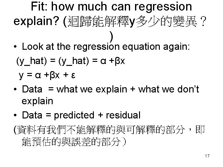
Fit: how much can regression explain? (迴歸能解釋y多少的變異？ ) • Look at the regression equation again: (y_hat) = α +βx y = α +βx + ε • Data = what we explain + what we don’t explain • Data = predicted + residual (資料有我們不能解釋的與可解釋的部分，即 能預估的與誤差的部分） 17

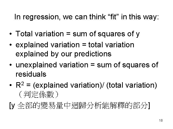
In regression, we can think “fit” in this way: • Total variation = sum of squares of y • explained variation = total variation explained by our predictions • unexplained variation = sum of squares of residuals • R 2 = (explained variation)/ (total variation) （判定係數） [y 全部的變易量中迴歸分析能解釋的部分] 18

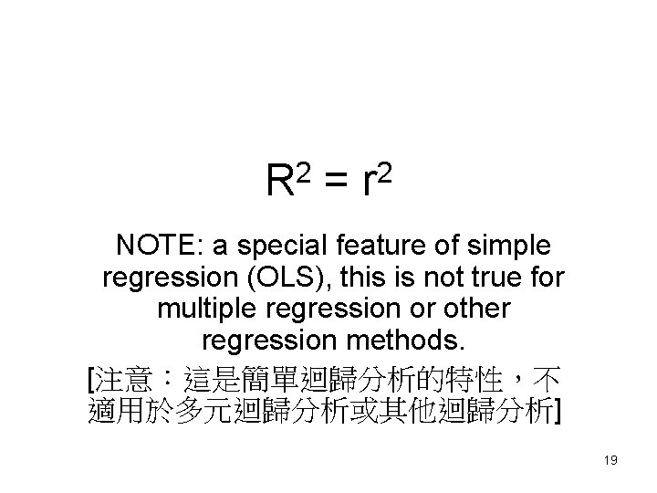
2 R = 2 r NOTE: a special feature of simple regression (OLS), this is not true for multiple regression or other regression methods. [注意：這是簡單迴歸分析的特性，不 適用於多元迴歸分析或其他迴歸分析] 19

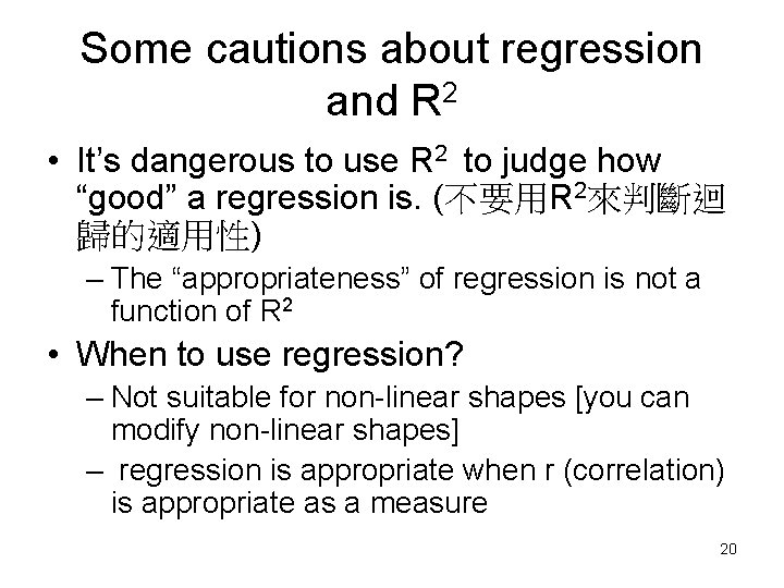
Some cautions about regression and R 2 • It’s dangerous to use R 2 to judge how “good” a regression is. (不要用R 2來判斷迴 歸的適用性) – The “appropriateness” of regression is not a function of R 2 • When to use regression? – Not suitable for non-linear shapes [you can modify non-linear shapes] – regression is appropriate when r (correlation) is appropriate as a measure 20

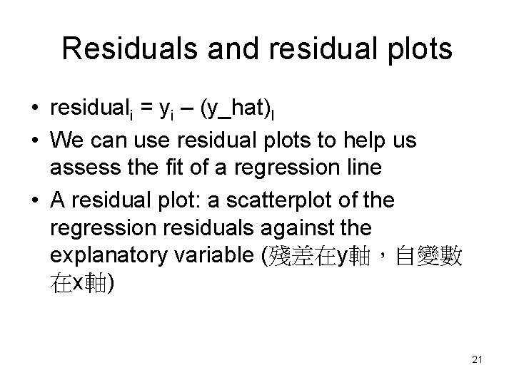
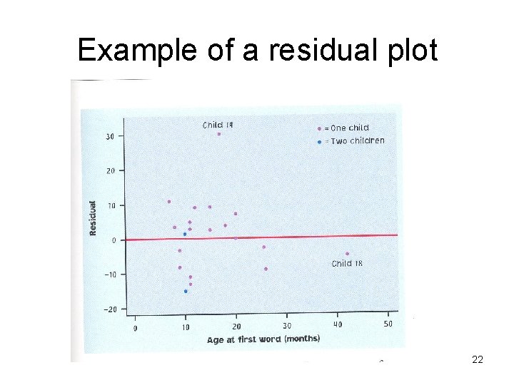
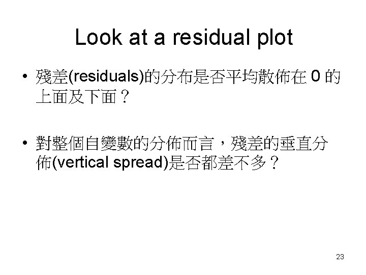
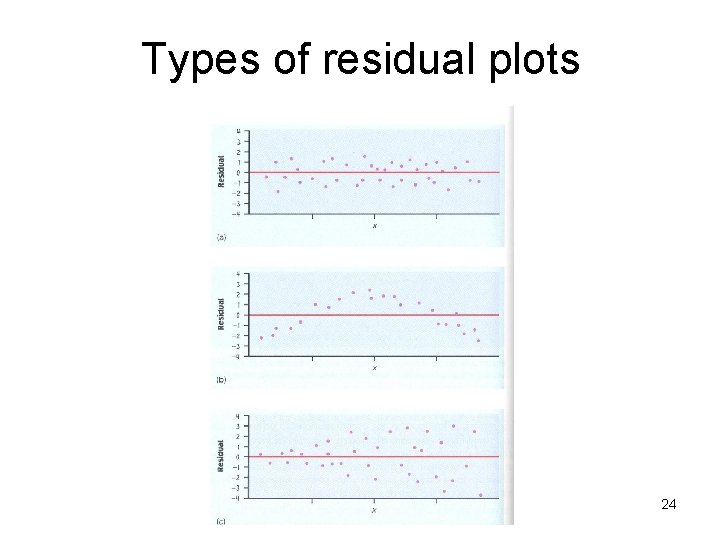
Residuals and residual plots • residuali = yi – (y_hat)I • We can use residual plots to help us assess the fit of a regression line • A residual plot: a scatterplot of the regression residuals against the explanatory variable (殘差在y軸，自變數 在x軸) 21

Example of a residual plot 22

Types of residual plots 24

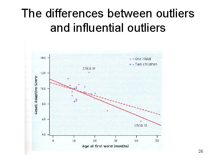
Outliers and influences • Outlier (極端值): a point that falls outside the overall patterns of the graph • Influential observation (深具影響的觀察值) = a point which, if removed, would markedly change the position of the regression line • NOTE: Outliers are not necessarily influential. 25

The differences between outliers and influential outliers 26

Outliers and influential observations • Outliers which are at the extremes of x are more likely to be influential than those are at the extremes of y (自變數的極端值比依 變數的極端值較有可能是對迴歸影響力大 的觀察值) • It is often a good idea to eliminate any influential outliers and recompute our regression without them. (建議: 將對迴歸影 響力大的觀察值刪除，再計算一次迴歸線) 27

Cautions about correlation and regression: • Extrapolation is not appropriate • Regression: pay attention to lurking or omitted variables – Lurking (omitted) variables: having influence on the relationship between two variables but is not included among the variables studied – A problem in establishing causation • Association does not imply causation. – Association alone: weak evidence about causation – Experiments with random assignment are the best way to establish causation. 28