Sharif University of Technology Wireless Communication Cellular Systems

Sharif University of Technology Wireless Communication Cellular Systems Fall 1395 Afshin Hemmatyar

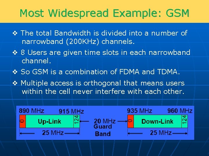
Most Widespread Example: GSM v The total Bandwidth is divided into a number of narrowband (200 KHz) channels. v 8 Users are given time slots in each narrowband channel. v So GSM is a combination of FDMA and TDMA. v Multiple access is orthogonal that means users within the cell never interfere with each other.

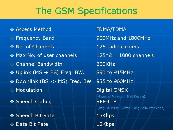
The GSM Specifications v Access Method FDMA/TDMA v Frequency Band 900 MHz and 1800 MHz v No. of Channels 125 radio carriers v Max No. of user channels 125*8 = 1000 channels v Channel Bandwidth 200 KHz v Uplink (MS BS) Freq. BW. 890 to 915 MHz v Downlink (BS -> MS) Freq. BW 935 to 960 MHz v Modulation Digital GMSK (Gaussian Minimum Shift Keying) v Speech Coding RPE-LTP (Regular Pulse Excited- Long Term Prediction) v Speech Bit Rate 13 Kbps v Data Bit Rate 12 Kbps

Why We Use Cellular Systems? v Assume we have S frequency channels available for our mobile system. v For GSM, we have 125 frequency channels and 8 time slots per channel thus S is equal to 1000. v How many people can speak at the same time in a city with that many channels? v If we use 1000 channels for the whole city with one Base station then obviously 1000 people can talk at the same time. v Then, how many people are actually speaking simultaneously with their phones in Tehran?

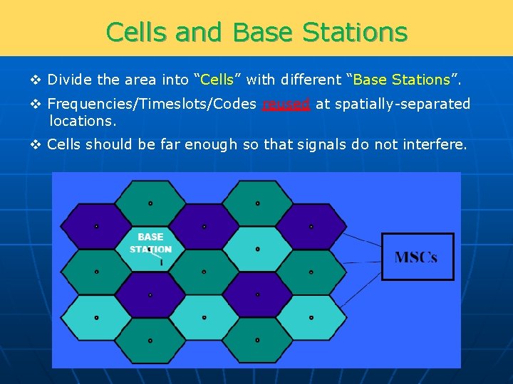
Cells and Base Stations v Divide the area into “Cells” with different “Base Stations”. v Frequencies/Timeslots/Codes reused at spatially-separated locations. v Cells should be far enough so that signals do not interfere.

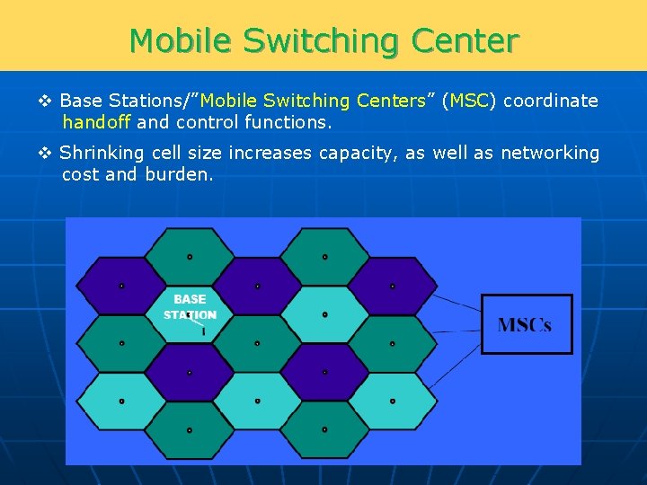
Mobile Switching Center v Base Stations/”Mobile Switching Centers” (MSC) coordinate handoff and control functions. v Shrinking cell size increases capacity, as well as networking cost and burden.

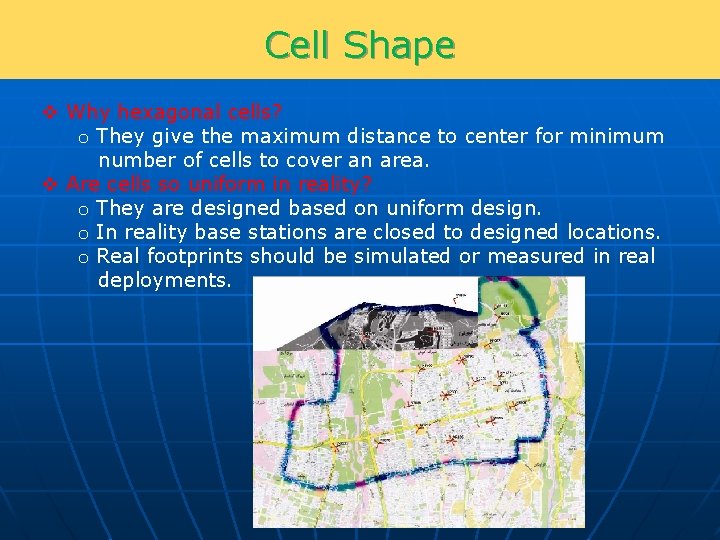
Cell Shape v Why hexagonal cells? o They give the maximum distance to center for minimum number of cells to cover an area. v Are cells so uniform in reality? o They are designed based on uniform design. o In reality base stations are closed to designed locations. o Real footprints should be simulated or measured in real deployments.

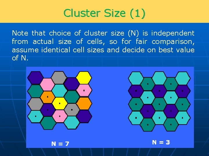
Reuse Concept v S: Total number of channels v K: Number of channels in each cell v N: Number of cells that in total use all S channels v N cells form a “cluster” v N is usually 1, 3, 4, 7, or 12

Cluster Size (1) Note that choice of cluster size (N) is independent from actual size of cells, so for fair comparison, assume identical cell sizes and decide on best value of N.

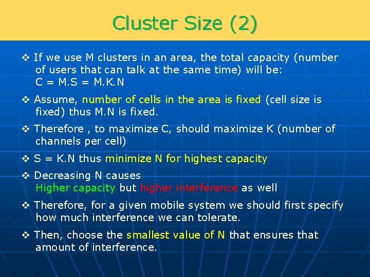
Cluster Size (2) v If we use M clusters in an area, the total capacity (number of users that can talk at the same time) will be: C = M. S = M. K. N v Assume, number of cells in the area is fixed (cell size is fixed) thus M. N is fixed. v Therefore , to maximize C, should maximize K (number of channels per cell) v S = K. N thus minimize N for highest capacity v Decreasing N causes Higher capacity but higher interference as well v Therefore, for a given mobile system we should first specify how much interference we can tolerate. v Then, choose the smallest value of N that ensures that amount of interference.

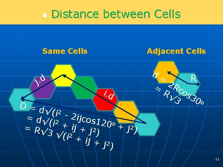
n Distance between Cells Same Cells j. d Adjacent Cells d i. d D=d √(i 2 = d√ 2 2 ijcos 1 (i + 20 o + 2 i j + j 2 = R√ j ) ) 3 √(i 2 + ij + 2 j ) = R = 2 Rc R√ os 3 30 o 11

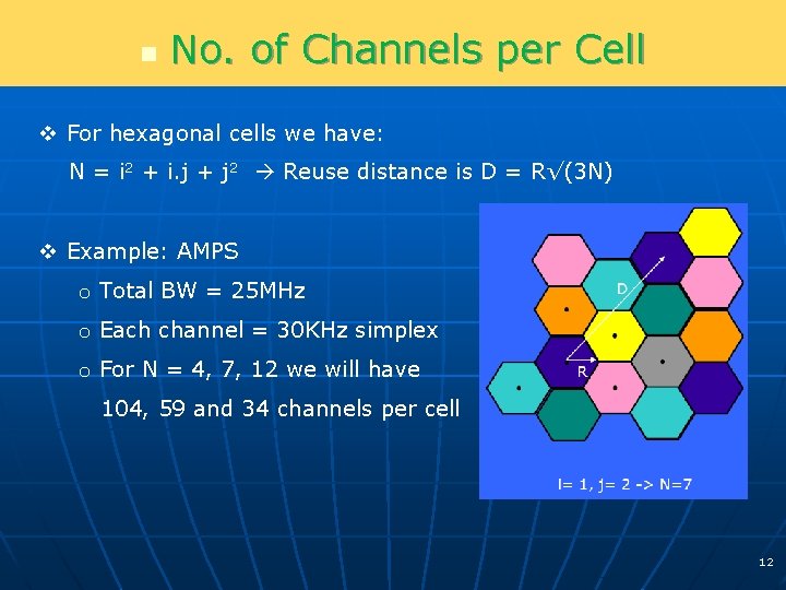
n No. of Channels per Cell v For hexagonal cells we have: N = i 2 + i. j + j 2 Reuse distance is D = R√(3 N) v Example: AMPS o Total BW = 25 MHz o Each channel = 30 KHz simplex o For N = 4, 7, 12 we will have 104, 59 and 34 channels per cell 12

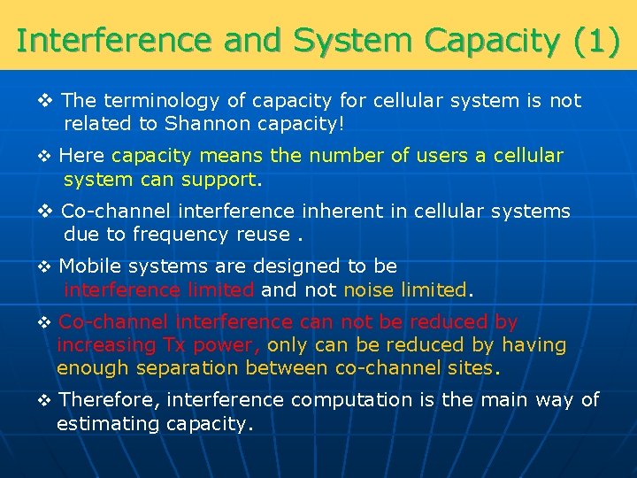
Interference and System Capacity (1) v The terminology of capacity for cellular system is not related to Shannon capacity! v Here capacity means the number of users a cellular system can support. v Co-channel interference inherent in cellular systems due to frequency reuse. v Mobile systems are designed to be interference limited and not noise limited. v Co-channel interference can not be reduced by increasing Tx power, only can be reduced by having enough separation between co-channel sites. v Therefore, interference computation is the main way of estimating capacity.

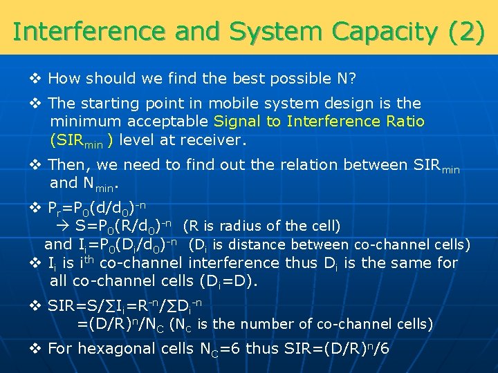
Interference and System Capacity (2) v How should we find the best possible N? v The starting point in mobile system design is the minimum acceptable Signal to Interference Ratio (SIRmin ) level at receiver. v Then, we need to find out the relation between SIRmin and Nmin. v Pr=P 0(d/d 0)-n S=P 0(R/d 0)-n (R is radius of the cell) and Ii=P 0(Di/d 0)-n (Di is distance between co-channel cells) v Ii is ith co-channel interference thus Di is the same for all co-channel cells (Di=D). v SIR=S/∑Ii=R-n/∑Di-n =(D/R)n/NC (NC is the number of co-channel cells) v For hexagonal cells NC=6 thus SIR=(D/R)n/6

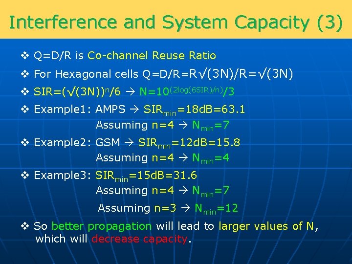
Interference and System Capacity (3) v Q=D/R is Co-channel Reuse Ratio v For Hexagonal cells Q=D/R=R√(3 N)/R=√(3 N) v SIR=(√(3 N))n/6 N=10(2 log(6 SIR)/n)/3 v Example 1: AMPS SIRmin=18 d. B=63. 1 Assuming n=4 Nmin=7 v Example 2: GSM SIRmin=12 d. B=15. 8 Assuming n=4 Nmin=4 v Example 3: SIRmin=15 d. B=31. 6 Assuming n=4 Nmin=7 Assuming n=3 Nmin=12 v So better propagation will lead to larger values of N, which will decrease capacity.

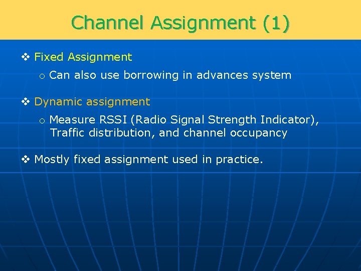
Channel Assignment (1) v Fixed Assignment o Can also use borrowing in advances system v Dynamic assignment o Measure RSSI (Radio Signal Strength Indicator), Traffic distribution, and channel occupancy v Mostly fixed assignment used in practice.

Channel Assignment (2) v In reality, channel planning is a complex optimization problem, that need to use special program. v Part of mobile channels are devoted to signaling. Thus we should to use better reuse ratio (for example 12 instead of 7) v In CDMA systems in theory, reuse ratio “ 1” can be used. v In practice, we don’t assign co-channel frequencies to neighboring cells to control interference levels. v Also an “equivalent reuse ratio” can be defined for CDMA systems.

Adjacent Channel Interference (1) v If Rx filters were ideal then “Adjacent Channel Interference” was not important. v But in reality filters are not ideal and so adjacent channel signals may also enter the receiver. v Highest Adjacent Channel Interference when desired user at cell boundaries. v In practice Adjacent channels are not used in the same cell or even in neighboring cells.

Adjacent Channel Interference (2) v Example: o In same cell scenario, if another user is much closer to the base than the desired user, its adjacent channel signal can cause significant interference. o Assume the ratio of distance from the two sources to the base (D 1/D 2), is equal to 20, then SIR =20 -n which for n=4 is equal to -52 d. B. o If Rx filter slope is 20 d. B/oct, at least 6 channel separation (each 200 KHz) between users is required. v In practice some sort of “power control” is used (more important in CDMA).

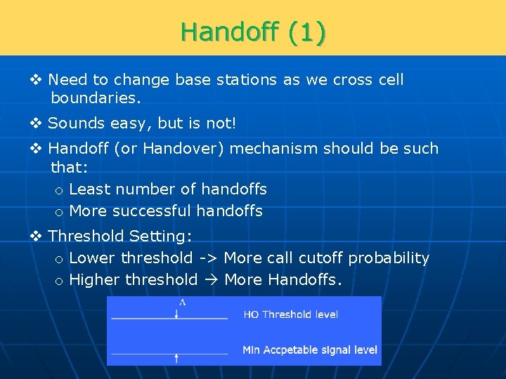
Handoff (1) v Need to change base stations as we cross cell boundaries. v Sounds easy, but is not! v Handoff (or Handover) mechanism should be such that: o Least number of handoffs o More successful handoffs v Threshold Setting: o Lower threshold -> More call cutoff probability o Higher threshold More Handoffs.

Handoff (2) v Signals should also be averaged over time, otherwise signals get disconnected due to fading. v Should also consider velocity in Handoff process. v Should monitor other Base Station signals as well. v Channel Reservation for Handoff v Soft Handoff in CDMA systems.

Trunking Theory (1) v Lets assume we have to cover a city with our mobile system. v Simple question: For a given number of subscribers, how many channels should we assign to that area? v In practice, for a telephony system when you want to cover N subscribers, you do not assign N channel to them. This is due to the fact that subscribers connect to network only occasionally. v For example, in an office with N employees, the number of lines that talk at the same time is only a fraction of N. v Obviously we need to define an acceptable quality level that based on that we can find required number of channels for a given N.

Trunking Theory (2) v Trunking concept: Allowing large number of users to share relatively small number of channels based on the fact users use the channel statistically over time v Based on a quantitative measure of acceptable service, N can be found. v Acceptable service quality in trunking theory is defined based on the measureable “Grade of Service” (Go. S)_ parameter. v Go. S is usually defined based on the following two parameters: o “Blocking Rate” which is the probability of getting a busy tone when trying to dial a number. o “Waiting Period” to get the number through (for queued systems).

Trunking Theory (3) v Basic definition: Ø Blocked Call: A call that can not get through Ø Holding Time: Average duration of a call (H in sec) Ø Request Rate: Average number of requested calls in unit of time for each user (λ in 1/sec) Ø Erlang: One Erlang is the amount of traffic that will completely occupy the channel for the given period of time. Example: If a channel in one hour is only occupied for 30 minutes then the traffic of that channel is 0. 5 Erlangs. Ø Traffic Intensity: Average occupancy of one or more channel (A in Erlangs) Ø Go. S: o Possibility of blockage of a call (Erlang B formula) o Possibility of a connection with a delay more than a specific value (Erlang C formula)

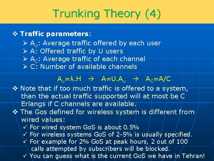
Trunking Theory (4) v Traffic parameters: Ø Au: Average traffic offered by each user Ø A: Offered traffic by U users Ø AC: Average traffic of each channel Ø C: Number of available channels Au=λ. H A=U. Au AC=A/C v Note that if too much traffic is offered to a system, than the actual traffic supported will at most be C Erlangs if C channels are available. v The Gos defined for wireless system is different from wired values: ü For wired system Go. S is about 0. 5% ü For wireless systems Go. S of 2 -5% is usually specified. ü For example for 2% Go. S at peak hours, 2 out of 100 calls attempted by subscribers will be blocked. ü You can guess what is the current Go. S we have in Tehran!

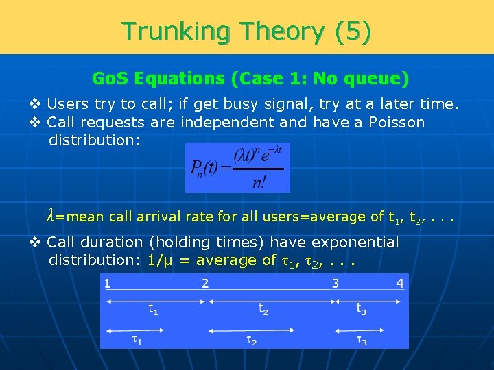
Trunking Theory (5) Go. S Equations (Case 1: No queue) v Users try to call; if get busy signal, try at a later time. v Call requests are independent and have a Poisson distribution: λ=mean call arrival rate for all users=average of t 1, t 2, . . . v Call duration (holding times) have exponential distribution: 1/μ = average of τ1, τ2, . . .

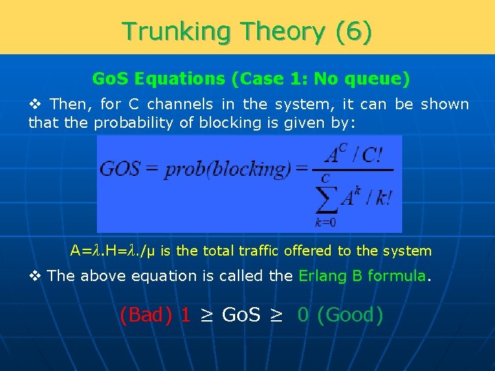
Trunking Theory (6) Go. S Equations (Case 1: No queue) v Then, for C channels in the system, it can be shown that the probability of blocking is given by: A=λ. H=λ. /μ is the total traffic offered to the system v The above equation is called the Erlang B formula. (Bad) 1 ≥ Go. S ≥ 0 (Good)

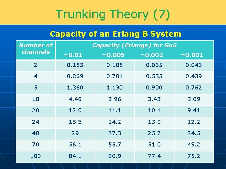
Trunking Theory (7) Capacity of an Erlang B System Number of channels Capacity (Erlangs) for Go. S =0. 01 =0. 005 =0. 002 =0. 001 2 0. 153 0. 105 0. 065 0. 046 4 0. 869 0. 701 0. 535 0. 439 5 1. 360 1. 130 0. 900 0. 762 10 4. 46 3. 96 3. 43 3. 09 20 12. 0 11. 1 10. 1 9. 41 24 15. 3 14. 2 13. 0 12. 2 40 29 27. 3 25. 7 24. 5 70 56. 1 53. 7 51. 0 49. 2 100 84. 1 80. 9 77. 4 75. 2

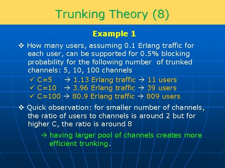
Trunking Theory (8) Example 1 v How many users, assuming 0. 1 Erlang traffic for each user, can be supported for 0. 5% blocking probability for the following number of trunked channels: 5, 100 channels ü C=5 1. 13 Erlang traffic 11 users ü C=10 3. 96 Erlang traffic 39 users ü C=100 80. 9 Erlang traffic 809 users v Quick observation: for smaller number of channels, the ratio of users to channels is around 2 but for higher C, the ratio is around 8 having larger pool of channels creates more efficient trunking.

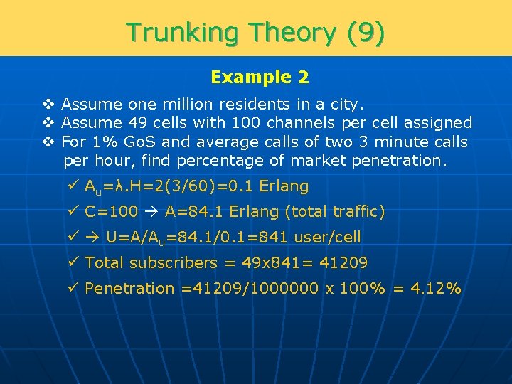
Trunking Theory (9) Example 2 v Assume one million residents in a city. v Assume 49 cells with 100 channels per cell assigned v For 1% Go. S and average calls of two 3 minute calls per hour, find percentage of market penetration. ü Au=λ. H=2(3/60)=0. 1 Erlang ü C=100 A=84. 1 Erlang (total traffic) ü U=A/Au=84. 1/0. 1=841 user/cell ü Total subscribers = 49 x 841= 41209 ü Penetration =41209/1000000 x 100% = 4. 12%

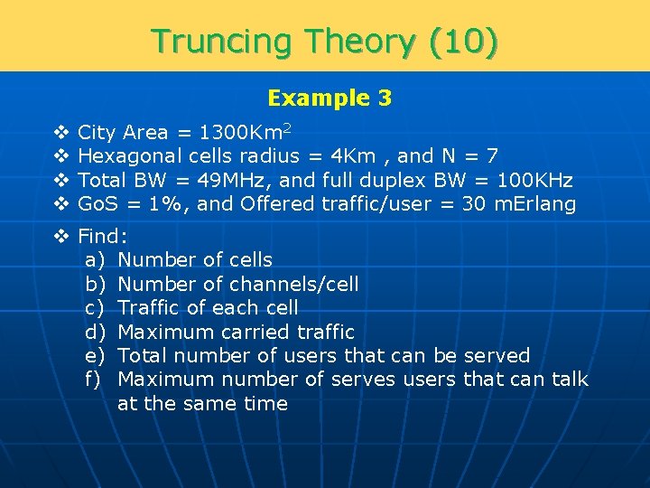
Truncing Theory (10) Example 3 v v City Area = 1300 Km 2 Hexagonal cells radius = 4 Km , and N = 7 Total BW = 49 MHz, and full duplex BW = 100 KHz Go. S = 1%, and Offered traffic/user = 30 m. Erlang v Find: a) Number of cells b) Number of channels/cell c) Traffic of each cell d) Maximum carried traffic e) Total number of users that can be served f) Maximum number of serves users that can talk at the same time

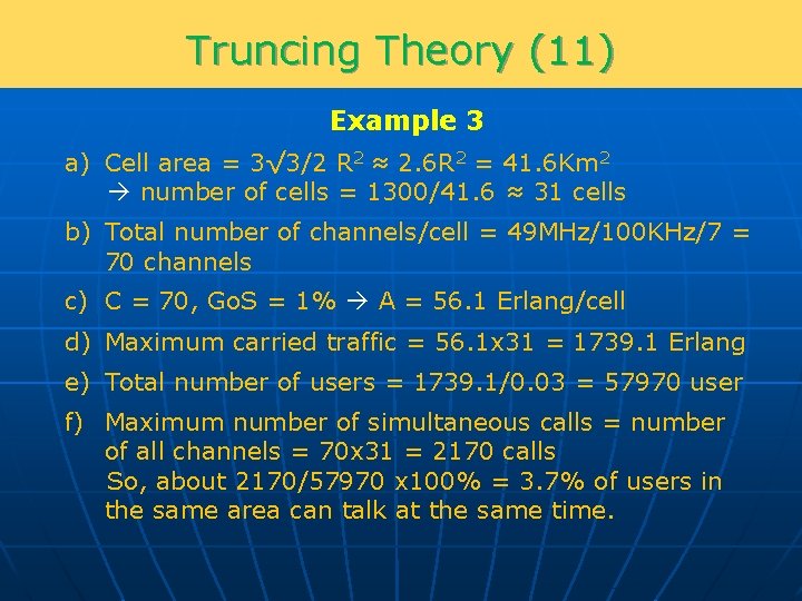
Truncing Theory (11) Example 3 a) Cell area = 3√ 3/2 R 2 ≈ 2. 6 R 2 = 41. 6 Km 2 number of cells = 1300/41. 6 ≈ 31 cells b) Total number of channels/cell = 49 MHz/100 KHz/7 = 70 channels c) C = 70, Go. S = 1% A = 56. 1 Erlang/cell d) Maximum carried traffic = 56. 1 x 31 = 1739. 1 Erlang e) Total number of users = 1739. 1/0. 03 = 57970 user f) Maximum number of simultaneous calls = number of all channels = 70 x 31 = 2170 calls So, about 2170/57970 x 100% = 3. 7% of users in the same area can talk at the same time.

Trunking Theory (12) Go. S Equations (Case 2: Blocked users queued) v In this scenario, blocked users will enter a queue. v The new model for such scenario is called Elrang C formula.

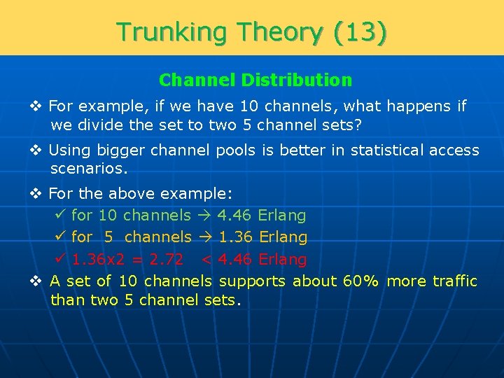
Trunking Theory (13) Channel Distribution v For example, if we have 10 channels, what happens if we divide the set to two 5 channel sets? v Using bigger channel pools is better in statistical access scenarios. v For the above example: ü for 10 channels 4. 46 Erlang ü for 5 channels 1. 36 Erlang ü 1. 36 x 2 = 2. 72 < 4. 46 Erlang v A set of 10 channels supports about 60% more traffic than two 5 channel sets.

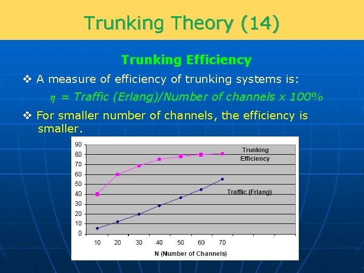
Trunking Theory (14) Trunking Efficiency v A measure of efficiency of trunking systems is: η = Traffic (Erlang)/Number of channels x 100% v For smaller number of channels, the efficiency is smaller.

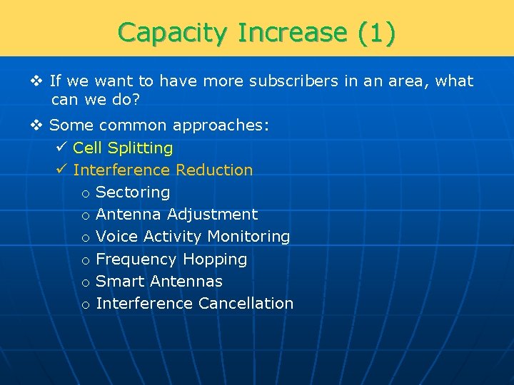
Capacity Increase (1) v If we want to have more subscribers in an area, what can we do? v Some common approaches: ü Cell Splitting ü Interference Reduction o Sectoring o Antenna Adjustment o Voice Activity Monitoring o Frequency Hopping o Smart Antennas o Interference Cancellation

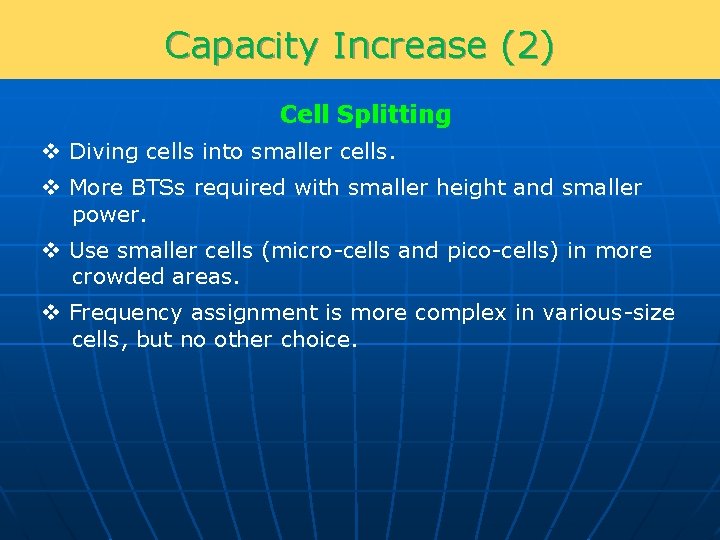
Capacity Increase (2) Cell Splitting v Diving cells into smaller cells. v More BTSs required with smaller height and smaller power. v Use smaller cells (micro-cells and pico-cells) in more crowded areas. v Frequency assignment is more complex in various-size cells, but no other choice.

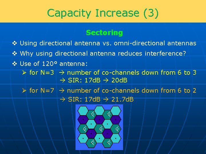
Capacity Increase (3) Sectoring v Using directional antenna vs. omni-directional antennas v Why using directional antenna reduces interference? v Use of 120° antenna: Ø for N=3 number of co-channels down from 6 to 3 SIR: 17 d. B 20 d. B Ø for N=7 number of co-channels down from 6 to 2 SIR: 17 d. B 21. 7 d. B

Capacity Increase (4) Sectoring SIR=(√(3 N))n/NC Omni Antenna NC= 6 120° Antenna NC= 2 60° Antenna NC= 1 v So, by sectoring can get higher SIR and so can use smaller N. v Disadvantages: o More equipment at BTS sites o More handoffs o Smaller trunking efficiency due to dividing channels in each cell into three groups (Erlang B formula) v In general, sectoring is widely used in practical mobile deployments.

Capacity Increase (5) Sectoring Example v Assume Go. S=1%, Avg. call duration=2 minutes, Avg. 1 call per hour, total number of channels =395, and N=7 v For omni antenna: 395/7 channel 44. 2 Erlang traffic 1326 call/hour v For 120° antenna: SIR increases by a factor of 3 for 7 -reuse 395/7/3 channels/sector 11. 2 Erlang/sector 33. 6 Erlang 1008 call/hour So, if we don’t change N, we improve SIR, but lose capacity. v For 60° antenna: SIR increases by a factor of 6 can reduce N from 7 to 4 395/4/6 channels/sector 9 Erlang/sector 54 Erlang 1620 call/hour So, if we can reduce N, by using sectored antenna, we may regain the lost trunking efficiency.

Capacity Increase (6) Other Means v Antenna height and tilt adjustment v Voice Activity ü Every user is only talking at about 40% of time ü V. A. is efficiency used in CDMA ü Also incorporated in GSM as DTX (discontinuous transmission) v Frequency Hopping ü Use a set of frequencies that can be swapped randomly over time, instead of one fixed channel. ü Widely used in GSM also improves resistance to fading. ü Two modes in GSM: Baseband Synthesized ü Hop rate is around 200 Hz (slow rate hopping). ü Since all channels are not used all the time statistically reduces the interference (~2 d. B lower SIR requirement). ü In theory, can marginally achieve N=1 (full reuse). ü In practice, N=3 and N=4 are common.

Summary v In a cellular design always pay attention to the roles of two main factors: ü Interference ü Cluster size, Trunking Efficiency and Capacity v A change in system may improve one but degrade another one. v In general, mobile planning and optimization is a quite complicated and time consuming task relying mainly on lots of experience.