Remote Sensing Classification Methods Introduction to Remote Sensing

Remote Sensing Classification Methods

§ Introduction to Remote Sensing Example Applications and Principles § § What is Classification? Explore and Classify an Image with Multi. Spec Questions…

Definitions Lillesand Kiefer (1994) – “The science and art of obtaining information …acquired by a device that is not in contact with the object…” CCRS Glossary – “A group of techniques for collecting image or other forms of data … from measurements made at a distance from the object, and the processing and analysis of the data. ”

Examples of Remotely Sensed Data § § § Weather Ocean Properties Physical Geography Major Disturbance Events / Hazards Cultural Features – urban mapping Many other examples – thematic info

back

disturbance back

back

Decision From Lillesand Kiefer (1994)

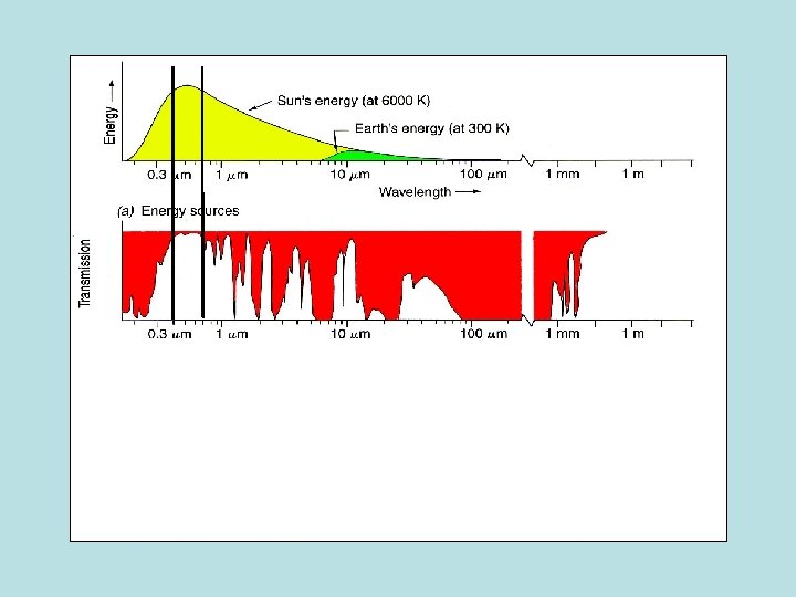
O 3 absorption at 0. 2 um

H 2 O absorption at 1. 4, 1. 6, and 1. 9 um

CO 2 absorption at 2. 0 um

CH 4 absorption at 2. 2 – 2. 5 um

Human eye

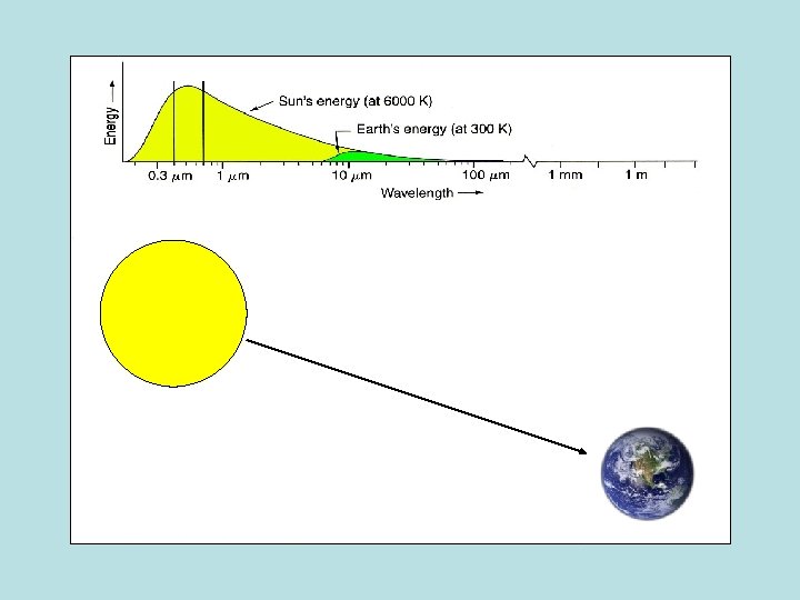
E(l)i – [ E(l)a + E(l)t ] = Er(l) Incident Energy Reflected Energy

Images vs. Maps

What are the characteristics of a thematic map? • Abstraction • Finite number of specified (discrete) classes • Scale (coarse) • Sharp boundaries – cartographic tradition, vector representation

Finite number of specified classes Generalize to a hierarchy of classes 1. Urban A. B. C. Residential Commercial Industrial 2. Agricultural A. B. C. Cropland Pasture Orchards 3. Etc…

Scale • Scale of map determines the scale (and detail) of classes 100 Pixel Size (meters) 10 1 I II III Level of Detail (Coarse to Fine)

Scale • Scale of imagery determines detail of what one sees – – Forest Community types Individual tree species Branches, leaf – – City Neighborhood Block House (roof) & Garden

Sharp boundaries • Sharp – Political boundary – Geological contact (unconformity) • Fuzzy – Vegetation community – Wetland to dry area In remote sensing: One class per pixel, and thus sharp boundaries

How to go from remote sensing data to classes? • Humans – strong pattern recognition ability – Spatial • • • Shape Size Context – Spectral • Relative brightness • Color • Remote Sensing – Usually purely spectral: each pixel classified independently

Snow Vs. Clouds

Snow Vs. Clouds scatter at all wavelengths Snow absorbs at >1. 4 mm c

Remote Sensing Pixel Data pixel 1, 1 = B 1 B 2 B 3. . . Bn z z z x x z x y y y y y z Band 2 Band 1 y = forest, x = agricultural field, z = natural grassland

Remote Sensing Pixel Data Decision Boundary pixel 1, 1 = B 1 B 2 B 3. . . Bn z z z x x z x y y y y y z Band 2 Band 1 y = forest, x = agricultural field, z = natural grassland

Classification Approaches • Supervised – Analyst identifies representative training sites for each informational class – Algorithm generates decision boundaries • Unsupervised – Algorithm identifies clusters in data – Analyst labels clusters

Supervised Classification Analyst identifies training areas for each informational class Algorithm identifies signatures (mean, variance, covariance, etc) Classify all pixels Informational Class Map

Unsupervised Classification Algorithm clusters data – find inherent classes Classify all pixels based on clusters Spectral class map Analyst labels clusters (May involve grouping of clusters) Informational class map

Labeling of classes • Bispectral plots Band 2 x x x y y Band 1 • “Spectral curves” • Classification map y

Spectral Classes Vs. Informational Classes Ideal Spectral classes A B Informational Classes 1 2 Concrete Reality Or A B C 1 A 1 2 3 4 B C 2 Fresh blacktop Old blacktop

Unsupervised Classification Methods • Histogram peak/valley finding • ISODATA – moving means

Histogram peak/valley finding Histogram of values in the image How many classes present? Frequency DN Value of Band x Assumptions: More pure pixels than mixed pixels Classes are distinctive

Histogram peak/valley finding Histogram of values in the image How many classes present? Frequency DN Value of Band x How do we identify significant peaks?

ISODATA Iterative Self Organizing Data Analysis Technique • More robust • User specifies – Iteration • Maximum # • Minimum change between iterations – Clusters • Maximum # (less usually found) • Starting locations (along diagonal, or 1 st PC, or arbitrary) – Splitting and merging parameters • Minimum # of pixels per cluster (e. g. 0. 01% of the data, then merge) • Maximum spread (e. g. if standard deviation large, then split)

ISODATA Classification: 1 Initial classification from arbitrary cluster centers Minimum distance to means classification rule x x Band 2 x x x x Total distance = 77 + x Arbitrary cluster centers + Band 1

ISODATA Classification: 2 Initial classification from arbitrary cluster centers Minimum distance to means classification rule x x + Band 2 x x + x x x Total distance = 54 x Adjusted cluster centers Band 1

ISODATA Classification: 3 Initial classification from arbitrary cluster centers x x Band 2 x x x + x x Band 1 + x Minimum distance to means classification rule Total distance = 26

ISODATA Classification: 4 Initial classification from arbitrary cluster centers x x Band 2 x x x + x x Band 1 + x Minimum distance to means classification rule Total distance = 18

ISODATA Classification: 4 Initial classification from arbitrary cluster centers x x Band 2 x x x + x x Band 1 + x Minimum distance to means classification rule Total distance = 18 No changes in pixels between classes, therefore stop

Multi. Spec RS Software • • Research and education Long period development and refinement Freely available Supported by tutorials http: //cobweb. ecn. purdue. edu/~biehl/Multi. Spec/