Radiative Transfer Theory at Optical and Microwavelengths applied

Radiative Transfer Theory at Optical and Microwavelengths applied to vegetation canopies: part 2 Uo. L MSc Remote Sensing course tutors: Dr Lewis Dr Saich plewis@geog. ucl. ac. uk psaich@geog. ucl. ac. uk

Radiative Transfer equation • Used extensively for (optical) vegetation since 1960 s (Ross, 1981) • Used for microwave vegetation since 1980 s

Radiative Transfer equation • Consider energy balance across elemental volume • Generally use scalar form (SRT) in optical • Generally use vector form (VRT) for microwave – includes polarisation using modified Stokes Vector and Mueller Matrix

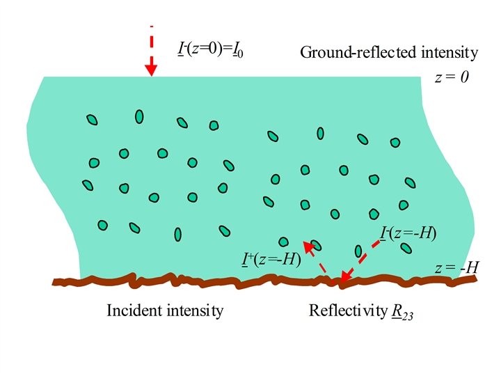
Medium 1: air z = l cos q 0=lm 0 q 0 Medium 2: canopy in air z Pathlength l Medium 3: soil Path of radiation

Scalar Radiative Transfer Equation • 1 -D scalar radiative transfer (SRT) equation – for a plane parallel medium (air) embedded with a low density of small scatterers – change in specific Intensity (Radiance) I(z, ) at depth z in direction wrt z:

Scalar RT Equation • Source Function: • m - cosine of the direction vector ( ) with the local normal – accounts for path length through the canopy • ke - volume extinction coefficient • P() is the volume scattering phase function

Vector RT equation • Source: • I - modified Stokes vector • ke - a 4 x 4 extinction matrix • phase function replaced by a (4 x 4) phase matrix (averages of Mueller matrix)

Extinction Coefficient and Beers Law • Volume extinction coefficient: – ‘total interaction cross section’ – ‘extinction loss’ – ‘number of interactions’ per unit length • a measure of attenuation of radiation in a canopy (or other medium). Beer’s Law

Extinction Coefficient and Beers Law No source version of SRT eqn

Extinction Coefficient and Beers Law • Definition: – Qe( ) - extinction cross section for a particle (units of m 2) – Nv - volume density (Np m-3) – can be defined for specific polarisation • subscript p for p-polarisation ().

Extinction Coefficient and Beers Law • Definition: – volume absorption and scattering coefficients

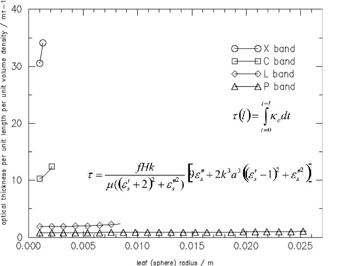
Optical Depth • Definition:

Single Scattering Albedo • Definition: • Effectively = reflectance + transmittance for optical • w(l)=rl(l)+tl(l)

Optical Extinction Coefficient for Oriented Leaves • Definition: extinction cross section:

Optical Extinction Coefficient for Oriented Leaves

Optical Extinction Coefficient for Oriented Leaves • range of G-functions small (0. 3 -0. 8) and smoother than leaf inclination distributions; • planophile canopies, G-function is high (>0. 5) for low zenith and low (<0. 5) for high zenith; • converse true for erectophile canopies; • G-function always close to 0. 5 between 50 o and 60 o • essentially invariant at 0. 5 over different leaf angle distributions at 57. 5 o.

Medium 1: air z = l cos q 0=lm 0 q 0 Medium 2: canopy in air z Pathlength l Medium 3: soil Path of radiation

Optical Extinction Coefficient for Oriented Leaves •

Optical Extinction Coefficient for Oriented Leaves • so, radiation at bottom of canopy for spherical: • for horizontal:

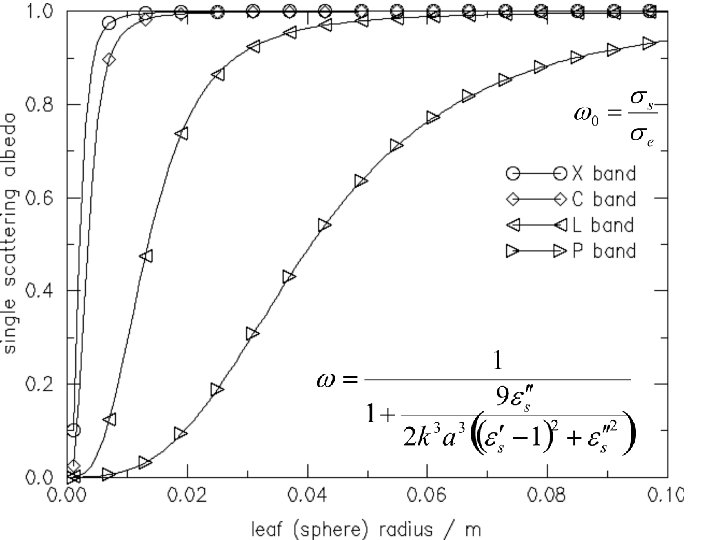
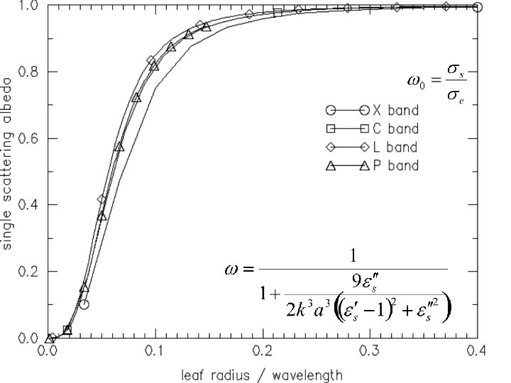
Extinction and Scattering in a Rayleigh Medium • Consider more general vector case • use example of Rayleigh medium – small spherical particles – can ‘modify’ terms for larger & non-spherical scatterers • e. g. discs, cylinders

Extinction and Scattering in a Rayleigh Medium • Scattering coefficient: • f - volume fraction of scatterers • es- is the dielectric constant of the sphere material • k is the wavenumber in air.

Extinction and Scattering in a Rayleigh Medium • Absorption coefficient: • f - volume fraction of scatterers • es- is the dielectric constant of the sphere material • k is the wavenumber in air.

Rayleigh Optical Thickness • For spherical scatterers: • extinction is scalar – no cross-polarisation terms

Rayleigh Phase Matrix

Solution to VRT Equation • Iterative method for low albedo • Do for Rayleigh here

Solution to VRT Equation

Solution to VRT Equation • Boundary Conditions:

Solution to VRT Equation • Rephrase as integral equations: T(-x)=e-x is an attenuation (extinction) term due to Beer’s Law

Insert boundary conditions VRT

VRT: upward terms

VRT: downward terms

Zero Order Solution • Set source terms in to zero:

First Order Solution • Iterative method: Insert zero-O solution as source

First Order Solution • Result: k 1= ke(1/m 0+1/ms); k 2= ke(1/m 0 -1/ms)

First Order Solution • Upward Backscattered Intensity at z=0

First Order Solution direct intensity reflected at canopy base, doubly attenuated through the canopy;

First Order Solution ‘double bounce’ term involving: a ground interaction, (downward) volumetric scattering by the canopy, additional ground interaction. Includes a double attenuation Term is generally very small and is often ignored.

First Order Solution downward volumetric scattering term, followed by a soil interaction, including a double attenuation on the upward and downward paths

First Order Solution Ground interaction followed by volumetric scattering by the canopy in the upward direction, again including double attenuation

First Order Solution Pure volumetric scattering by the canopy. ‘path radiance’

First Order Solution • Now have first order solution • Express as backscatter • plug in extinction coefficient & phase functions for Rayleigh – consider different scatterers – consider different soil scattering

Second+ Order Solution • 2+ solutions similarly obtained – set the first-order solutions as the source terms. – Note whilst no cross-polarisation terms for spherical (Rayleigh) scatterers, they do occur in second+ order scattering, • i. e. cross-polarisation for spherical scatterers is result of multiple scattering. – 2+ O used in RT 2 model (Saich)

A Scalar Radiative Transfer Solution • Attempt similar first Order Scattering solution – N. B. - mean different to microwave field – in optical, consider total number of interactions • with leaves + soil – in microwave, consider only canopy interactions • Already have extinction coefficient:

SRT • Phase function: • ul - leaf area density; • m’ - cosine of the incident zenith angle • G - area scattering phase function.

SRT • Area scattering phase function: • double projection, modulated by spectral terms

SRT • Phrase in scalar form of VRT: rsoil – soil directional reflectance factor

SRT • Insert Phase function definition: • so:

SRT • Note Joint Gap Probability:

SRT • Integrate to give intensity at z=0: • so:

Optical Extinction Coefficient • Insert into k 3:

SRT • Since the LAI, L=ul. H:

SRT: 1 st O mechanisms • through canopy, reflected from soil & back through canopy

SRT: 1 st O mechanisms Canopy only scattering Direct function of w Function of gl, L, and viewing and illumination angles

1 st O SRT • Special case of spherical leaf angle:

1 st O SRT • Further, linear function between leaf reflectance and transmittance:

Multiple Scattering • Albedo not always low (NIR) – cant use interative method – range of approximate solutions available

RT Modifications • Hot Spot – joint gap probabilty: Q – For far-field objects, treat incident & exitant gap probabilities independently – product of two Beer’s Law terms

RT Modifications • Consider retro-reflection direction: – assuming independent: – But should be:

RT Modifications • Consider retro-reflection direction: – But should be: – as ‘have already travelled path’ – so need to apply corrections for Q in RT • e. g.

RT Modifications • As result of finite object size, hot spot has angular width – depends on ‘roughness’ • leaf size / canopy height (Kuusk) • similar for soils • Also consider shadowing/shadow hiding

Summary • SRT / VRT formulations – extinction – scattering (source function) • Beer’s Law – exponential attenuation – rate - extinction coefficient • LAI x G-function for optical • considered Rayleigh for microwave

Summary • VRT 1 st O solution – 2 stream iterative approach – work 0 th-O solution – plug into VRT eqn – work 1 st-O solution – calculate for upward intensity at top of canopy – 5 scattering mechanisms

Summary • SRT 1 st O solution – similar, but 1 x canopy or 1 x soil solutions only – use area scattering phase function – simple solution for spherical leaf angle – 2 scattering mechanisms • Modification to SRT: – hot spot at optical