Querying the Internet with PIER PIER Peertopeer Information

Querying the Internet with PIER (PIER = Peer-to-peer Information Exchange and Retrieval) VLDB 2003 Ryan Huebsch, Joe Hellerstein, Nick Lanham, Boon Thau Loo, Timothy Roscoe, Scott Shenker, Ion Stoica p 2 p, Fall 05 1

What is PIER? A query engine that scales up to thousands of participating nodes = relational queries + DHT Built on top of a DHT Motivation, Why? In situ distributed querying (as opposed to warehousing) Network monitoring network intrusion detection: sharing and querying fingerprint information p 2 p, Fall 05 2

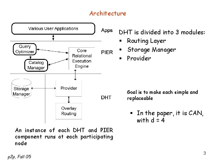
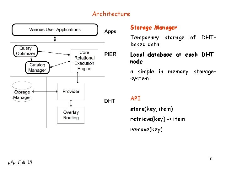
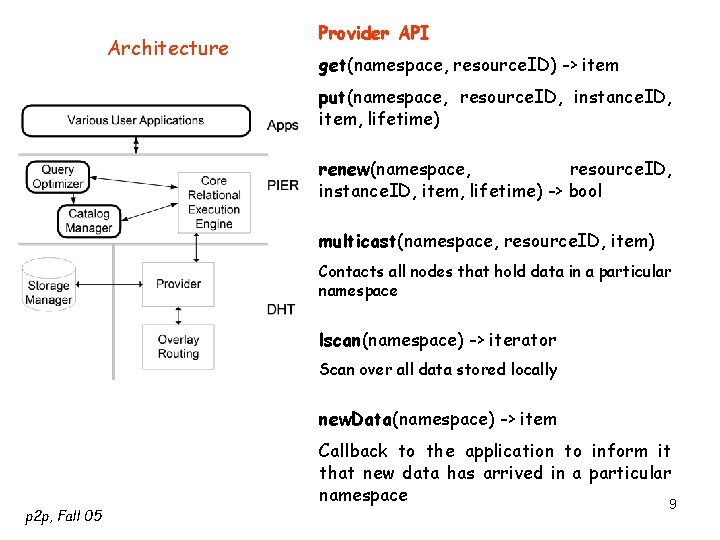
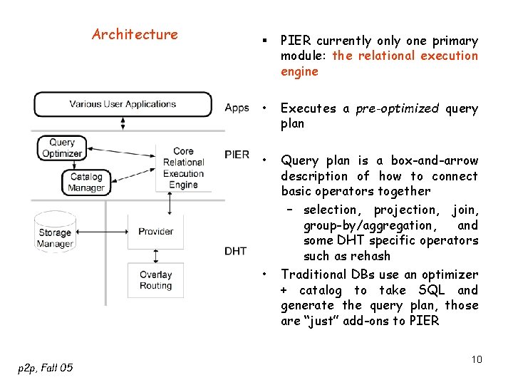
Architecture DHT is divided into 3 modules: § Routing Layer § Storage Manager § Provider Goal is to make each simple and replaceable § In the paper, it is CAN, with d = 4 An instance of each DHT and PIER component runs at each participating node p 2 p, Fall 05 3

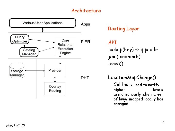
Architecture Routing Layer API lookup(key) -> ippaddr join(landmark) leave() Location. Map. Change() Callback used to notify higher levels asynchronously when a set of kwys mapped locally has changed p 2 p, Fall 05 4

Architecture Storage Manager Temporary storage of DHTbased data Local database at each DHT node a simple in memory storagesystem API store(key, item) retrieve(key) -> item remove(key) p 2 p, Fall 05 5

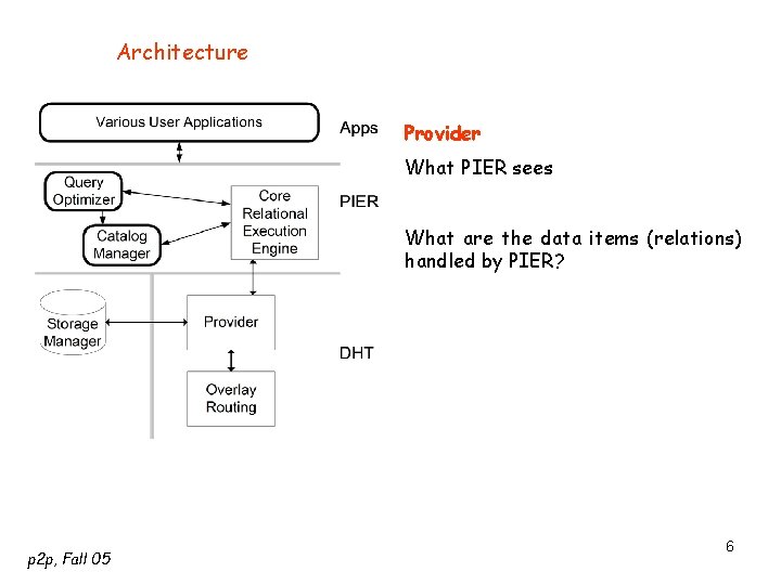
Architecture Provider What PIER sees What are the data items (relations) handled by PIER? p 2 p, Fall 05 6

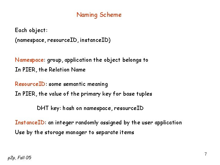
Naming Scheme Each object: (namespace, resource. ID, instance. ID) Namespace: group, application the object belongs to In PIER, the Relation Name Resource. ID: some semantic meaning In PIER, the value of the primary key for base tuples DHT key: hash on namespace, resource. ID Instance. ID: an integer randomly assigned by the user application Use by the storage manager to separate items p 2 p, Fall 05 7

Soft State Each object associated with a lifetime: how long should the DHT store the object To extend it, must use periodical RENEW calls p 2 p, Fall 05 8

Architecture Provider API get(namespace, resource. ID) -> item put(namespace, resource. ID, instance. ID, item, lifetime) renew(namespace, resource. ID, instance. ID, item, lifetime) -> bool multicast(namespace, resource. ID, item) Contacts all nodes that hold data in a particular namespace lscan(namespace) -> iterator Scan over all data stored locally new. Data(namespace) -> item p 2 p, Fall 05 Callback to the application to inform it that new data has arrived in a particular namespace 9

Architecture § PIER currently one primary module: the relational execution engine • Executes a pre-optimized query plan • Query plan is a box-and-arrow description of how to connect basic operators together – selection, projection, join, group-by/aggregation, and some DHT specific operators such as rehash Traditional DBs use an optimizer + catalog to take SQL and generate the query plan, those are “just” add-ons to PIER • p 2 p, Fall 05 10

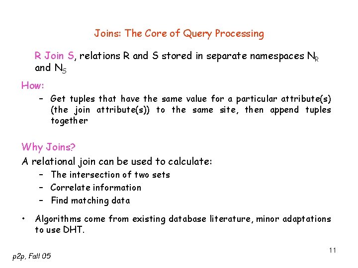
Joins: The Core of Query Processing R Join S, relations R and S stored in separate namespaces NR and NS How: – Get tuples that have the same value for a particular attribute(s) (the join attribute(s)) to the same site, then append tuples together Why Joins? A relational join can be used to calculate: – The intersection of two sets – Correlate information – Find matching data • Algorithms come from existing database literature, minor adaptations to use DHT. p 2 p, Fall 05 11

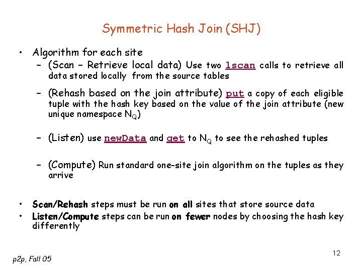
Symmetric Hash Join (SHJ) • Algorithm for each site – (Scan – Retrieve local data) Use two lscan calls to retrieve all data stored locally from the source tables – (Rehash based on the join attribute) put a copy of each eligible tuple with the hash key based on the value of the join attribute (new unique namespace NQ) – (Listen) use new. Data and get to NQ to see the rehashed tuples – (Compute) Run standard one-site join algorithm on the tuples as they arrive • • Scan/Rehash steps must be run on all sites that store source data Listen/Compute steps can be run on fewer nodes by choosing the hash key differently p 2 p, Fall 05 12

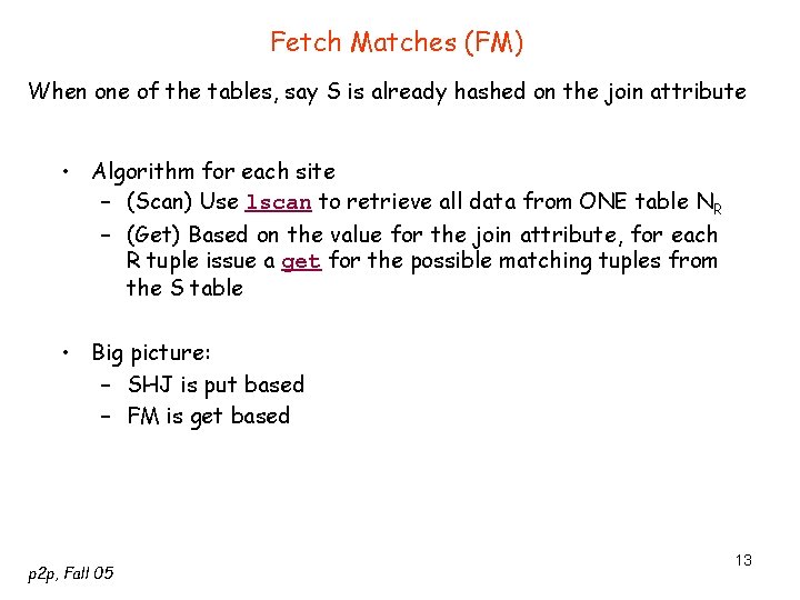
Fetch Matches (FM) When one of the tables, say S is already hashed on the join attribute • Algorithm for each site – (Scan) Use lscan to retrieve all data from ONE table NR – (Get) Based on the value for the join attribute, for each R tuple issue a get for the possible matching tuples from the S table • Big picture: – SHJ is put based – FM is get based p 2 p, Fall 05 13

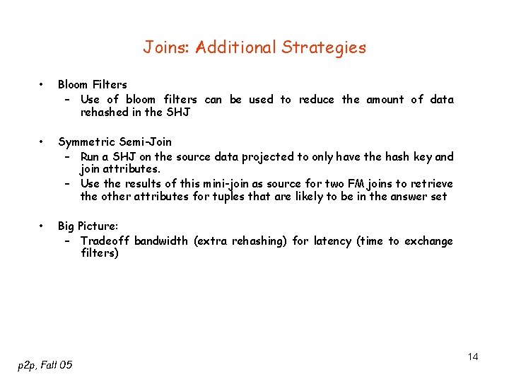
Joins: Additional Strategies • Bloom Filters – Use of bloom filters can be used to reduce the amount of data rehashed in the SHJ • Symmetric Semi-Join – Run a SHJ on the source data projected to only have the hash key and join attributes. – Use the results of this mini-join as source for two FM joins to retrieve the other attributes for tuples that are likely to be in the answer set • Big Picture: – Tradeoff bandwidth (extra rehashing) for latency (time to exchange filters) p 2 p, Fall 05 14

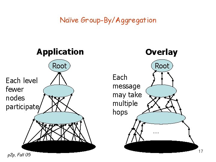
Naïve Group-By/Aggregation • A group-by/aggregation can be used to calculate: – Split data into groups based on value – Max, Min, Sum, Count, etc. • Goal: – Get tuples that have the same value for a particular attribute(s) (group-by attribute(s)) to the same site, then summarize data (aggregation). p 2 p, Fall 05 15

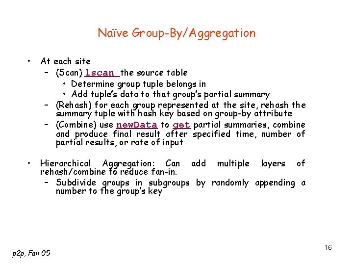
Naïve Group-By/Aggregation • At each site – (Scan) lscan the source table • Determine group tuple belongs in • Add tuple’s data to that group’s partial summary – (Rehash) for each group represented at the site, rehash the summary tuple with hash key based on group-by attribute – (Combine) use new. Data to get partial summaries, combine and produce final result after specified time, number of partial results, or rate of input • Hierarchical Aggregation: Can add multiple layers of rehash/combine to reduce fan-in. – Subdivide groups in subgroups by randomly appending a number to the group’s key p 2 p, Fall 05 16

Naïve Group-By/Aggregation Application Overlay Root Each message may take multiple hops Each level fewer nodes participate … Sources p 2 p, Fall 05 Sources 17

Codebase • Approximately 17, 600 lines of NCSS Java Code • Same code (overlay components/pier) run on the simulator or over a real network without changes • Runs simple simulations with up to 10 k nodes – Limiting factor: 2 GB addressable memory for the JVM (in Linux) • Runs on Millennium and Planet Lab up to 64 nodes – Limiting factor: Available/working nodes & setup time • Code: – Basic implementations of Chord and CAN – Selection, projection, joins (4 methods), and naïve aggregation. – Non-continuous queries p 2 p, Fall 05 18

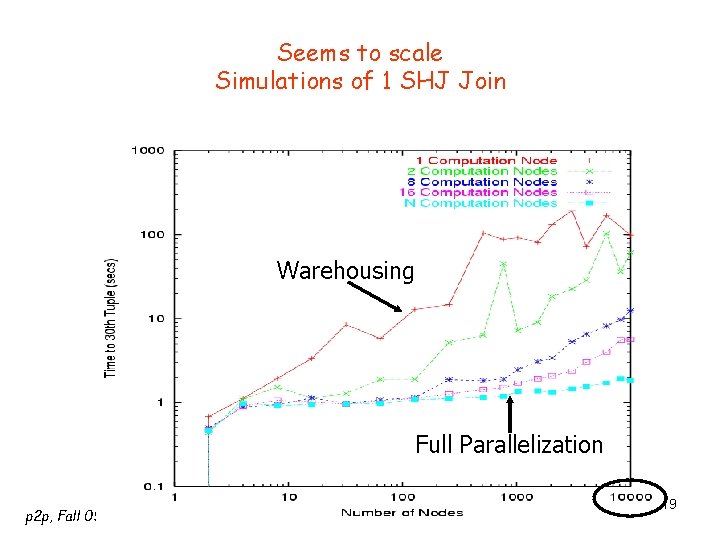
Seems to scale Simulations of 1 SHJ Join Warehousing Full Parallelization p 2 p, Fall 05 19

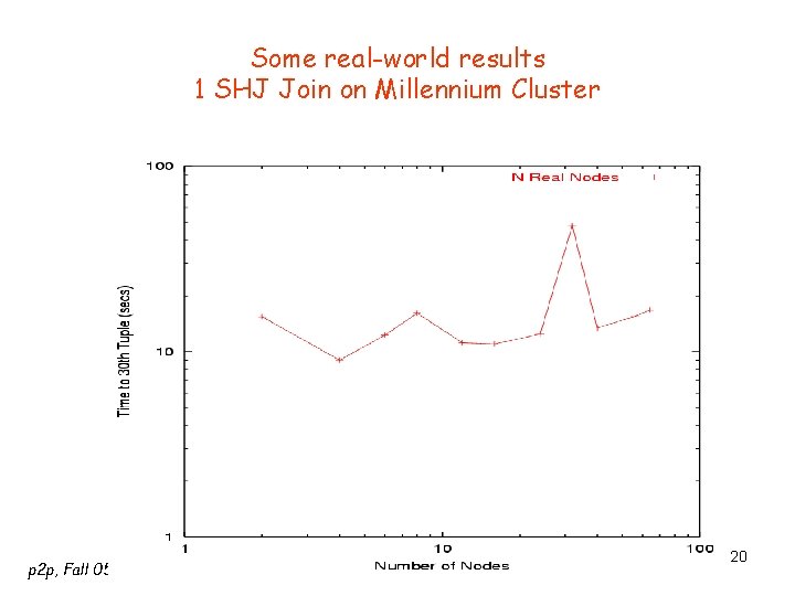
Some real-world results 1 SHJ Join on Millennium Cluster p 2 p, Fall 05 20