Query Processing Zachary G Ives University of Pennsylvania

Query Processing Zachary G. Ives University of Pennsylvania CIS 550 – Database & Information Systems

Making Use of the Data + Indices: Query Execution § § Query plans & exec strategies Basic principles Standard relational operators Querying XML 2

Making Use of the Data + Indices: Query Execution § § Query plans & exec strategies Basic principles Standard relational operators Querying XML 3

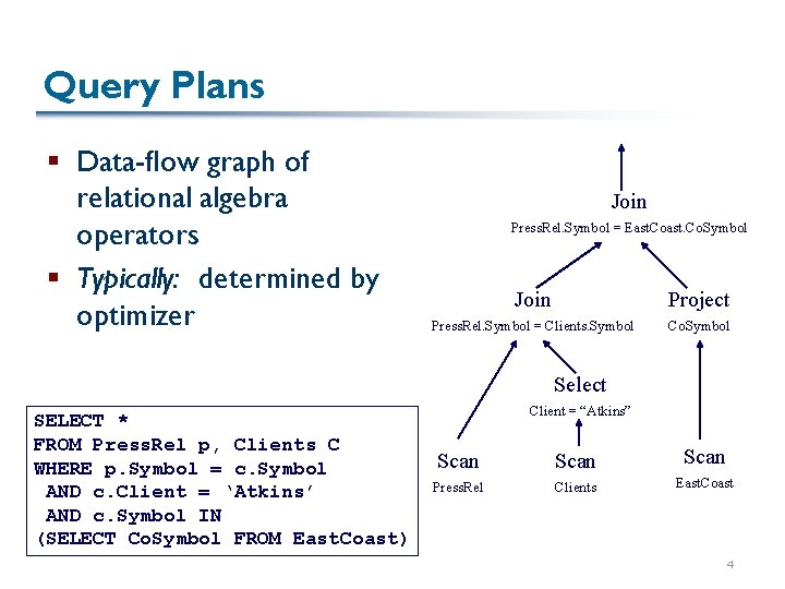
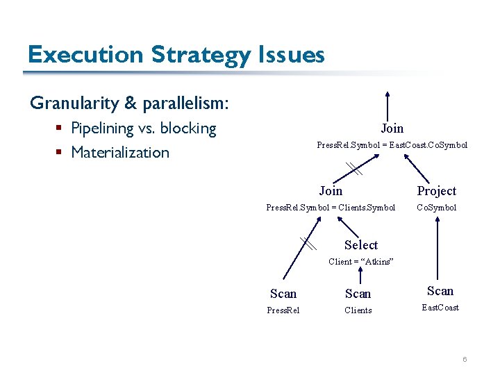
Query Plans § Data-flow graph of relational algebra operators § Typically: determined by optimizer Join Press. Rel. Symbol = East. Co. Symbol Join Project Press. Rel. Symbol = Clients. Symbol Co. Symbol Select SELECT * FROM Press. Rel p, Clients C WHERE p. Symbol = c. Symbol AND c. Client = ‘Atkins’ AND c. Symbol IN (SELECT Co. Symbol FROM East. Coast) Client = “Atkins” Scan Press. Rel Clients East. Coast 4

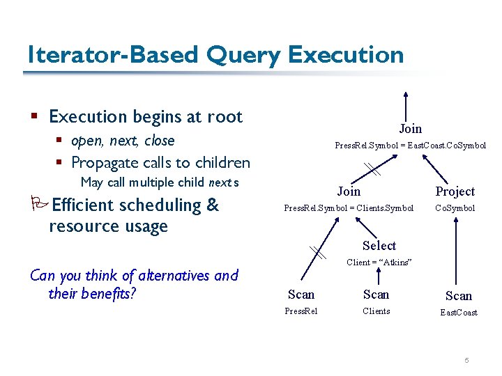
Iterator-Based Query Execution § Execution begins at root Join § open, next, close § Propagate calls to children Press. Rel. Symbol = East. Co. Symbol May call multiple child next s PEfficient scheduling & resource usage Join Project Press. Rel. Symbol = Clients. Symbol Co. Symbol Select Can you think of alternatives and their benefits? Client = “Atkins” Scan Press. Rel Clients East. Coast 5

Execution Strategy Issues Granularity & parallelism: § Pipelining vs. blocking § Materialization Join Press. Rel. Symbol = East. Co. Symbol Join Project Press. Rel. Symbol = Clients. Symbol Co. Symbol Select Client = “Atkins” Scan Press. Rel Clients East. Coast 6

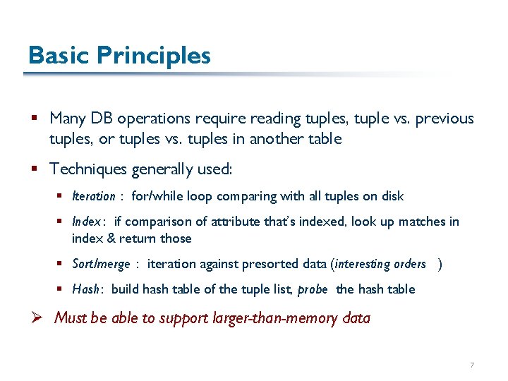
Basic Principles § Many DB operations require reading tuples, tuple vs. previous tuples, or tuples vs. tuples in another table § Techniques generally used: § Iteration : for/while loop comparing with all tuples on disk § Index : if comparison of attribute that’s indexed, look up matches in index & return those § Sort/merge : iteration against presorted data (interesting orders ) § Hash: build hash table of the tuple list, probe the hash table Ø Must be able to support larger-than-memory data 7

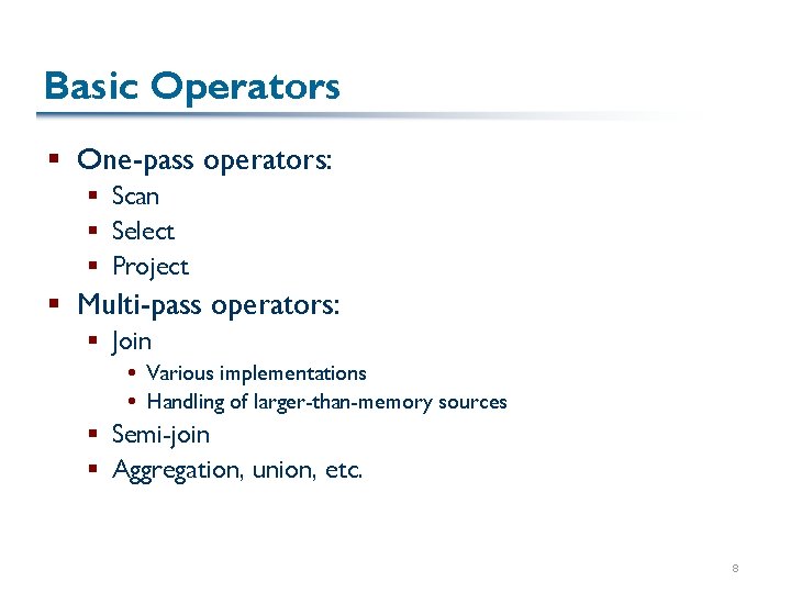
Basic Operators § One-pass operators: § Scan § Select § Project § Multi-pass operators: § Join Various implementations Handling of larger-than-memory sources § Semi-join § Aggregation, union, etc. 8

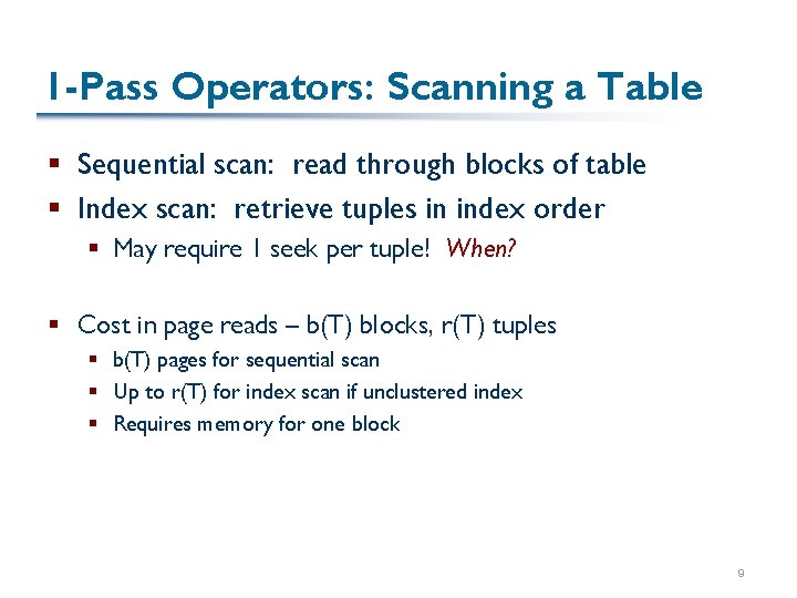
1 -Pass Operators: Scanning a Table § Sequential scan: read through blocks of table § Index scan: retrieve tuples in index order § May require 1 seek per tuple! When? § Cost in page reads – b(T) blocks, r(T) tuples § b(T) pages for sequential scan § Up to r(T) for index scan if unclustered index § Requires memory for one block 9

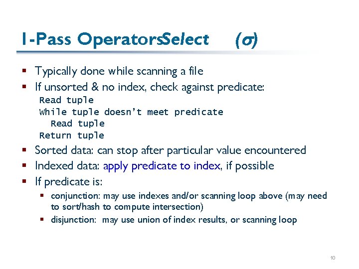
1 -Pass Operators: Select (s) § Typically done while scanning a file § If unsorted & no index, check against predicate: Read tuple While tuple doesn’t meet predicate Read tuple Return tuple § Sorted data: can stop after particular value encountered § Indexed data: apply predicate to index, if possible § If predicate is: § conjunction: may use indexes and/or scanning loop above (may need to sort/hash to compute intersection) § disjunction: may use union of index results, or scanning loop 10

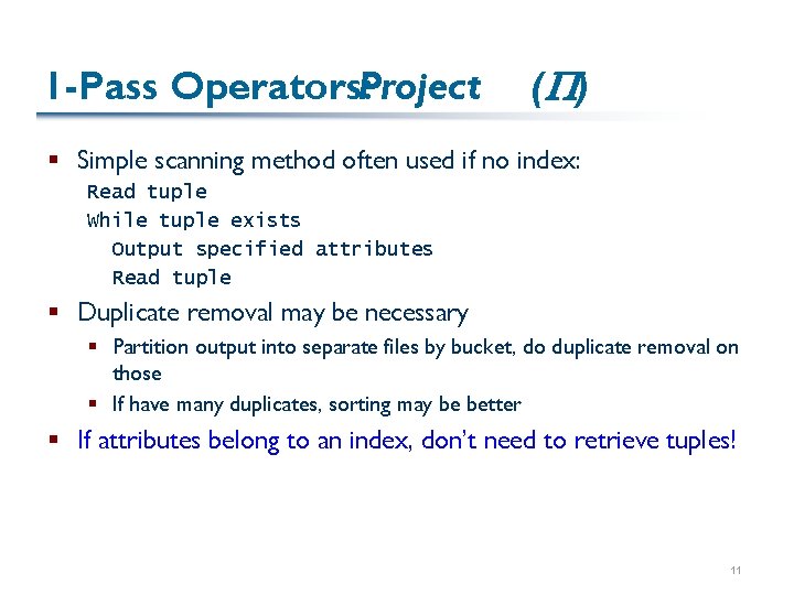
1 -Pass Operators: Project ( P) § Simple scanning method often used if no index: Read tuple While tuple exists Output specified attributes Read tuple § Duplicate removal may be necessary § Partition output into separate files by bucket, do duplicate removal on those § If have many duplicates, sorting may be better § If attributes belong to an index, don’t need to retrieve tuples! 11

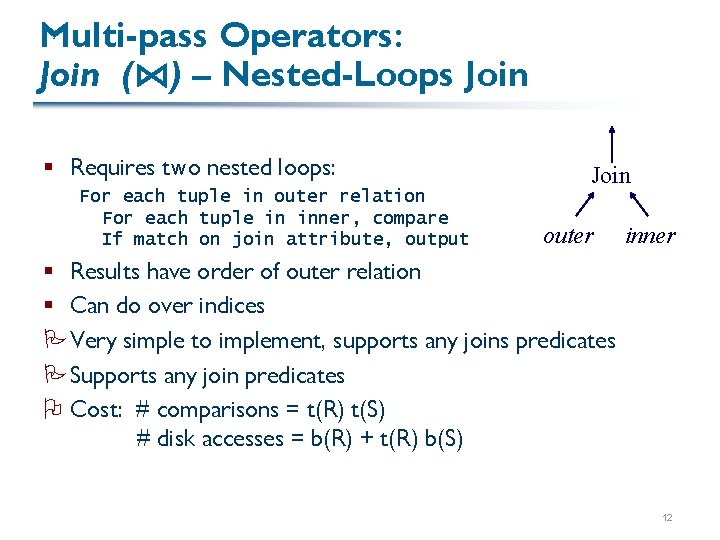
Multi-pass Operators: Join (⋈) – Nested-Loops Join § Requires two nested loops: For each tuple in outer relation For each tuple in inner, compare If match on join attribute, output Join outer inner § Results have order of outer relation § Can do over indices PVery simple to implement, supports any joins predicates PSupports any join predicates O Cost: # comparisons = t(R) t(S) # disk accesses = b(R) + t(R) b(S) 12

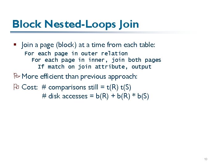
Block Nested-Loops Join § Join a page (block) at a time from each table: For each page in outer relation For each page in inner, join both pages If match on join attribute, output PMore efficient than previous approach: O Cost: # comparisons still = t(R) t(S) # disk accesses = b(R) + b(R) * b(S) 13

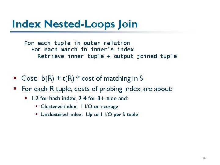
Index Nested-Loops Join For each tuple in outer relation For each match in inner’s index Retrieve inner tuple + output joined tuple § Cost: b(R) + t(R) * cost of matching in S § For each R tuple, costs of probing index are about: § 1. 2 for hash index, 2 -4 for B+-tree and: Clustered index: 1 I/O on average Unclustered index: Up to 1 I/O per S tuple 14

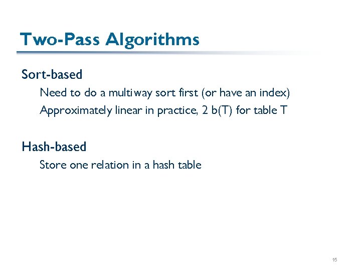
Two-Pass Algorithms Sort-based Need to do a multiway sort first (or have an index) Approximately linear in practice, 2 b(T) for table T Hash-based Store one relation in a hash table 15

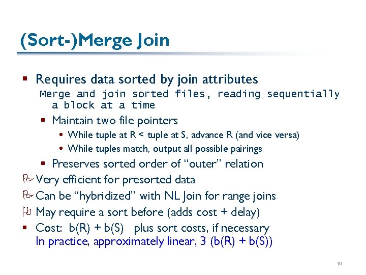
(Sort-)Merge Join § Requires data sorted by join attributes Merge and join sorted files, reading sequentially a block at a time § Maintain two file pointers While tuple at R < tuple at S, advance R (and vice versa) While tuples match, output all possible pairings § Preserves sorted order of “outer” relation PVery efficient for presorted data PCan be “hybridized” with NL Join for range joins O May require a sort before (adds cost + delay) § Cost: b(R) + b(S) plus sort costs, if necessary In practice, approximately linear, 3 (b(R) + b(S)) 16

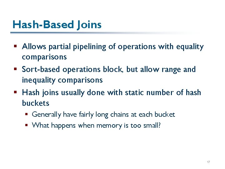
Hash-Based Joins § Allows partial pipelining of operations with equality comparisons § Sort-based operations block, but allow range and inequality comparisons § Hash joins usually done with static number of hash buckets § Generally have fairly long chains at each bucket § What happens when memory is too small? 17

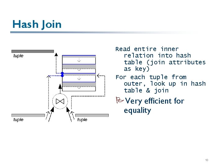
Hash Join Read entire inner relation into hash table (join attributes as key) For each tuple from outer, look up in hash table & join PVery efficient for equality 18

Running out of Memory § Resolution: When hash tables full Split hash table into files along bucket boundaries Partition remaining data in same way Recursively join partitions with diff. hash fn! § Hybrid hash join: flush “lazily” a few buckets at a time § Cost: <= 3 * (b(R) + b(S)) 19

Aggregation )( § Need to store entire table, coalesce groups with matching GROUP BY attributes § Compute aggregate function over group: § If groups are sorted or indexed, can iterate: Read tuples while attributes match, compute aggregate At end of each group, output result § Hash approach: Group together in hash table (leave space for agg values!) Compute aggregates incrementally or at end At end, return answers § Cost: b(t) pages. How much memory? 20

Other Operators § Duplicate removal very similar to grouping § All attributes must match § No aggregate § Union, difference, intersection: § Read table R, build hash/search tree § Read table S, add/discard tuples as required § Cost: b(R) + b(S) 21

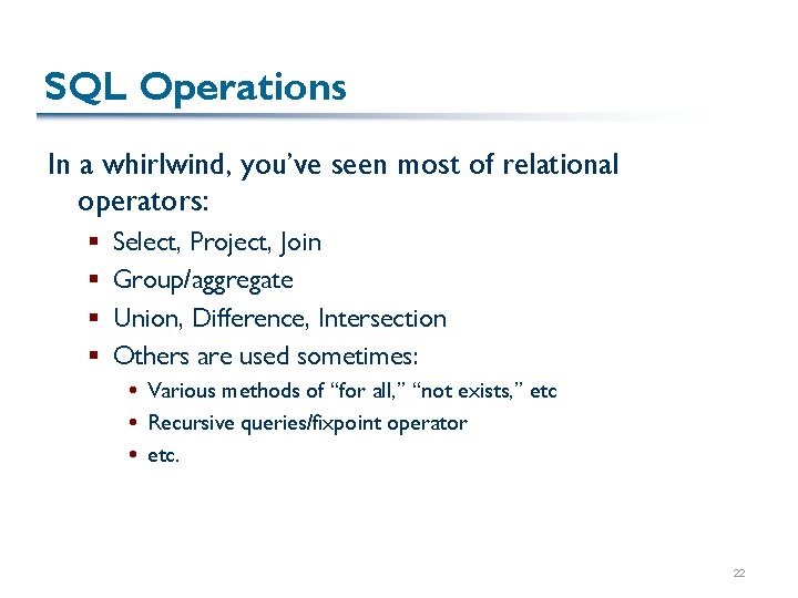
SQL Operations In a whirlwind, you’ve seen most of relational operators: § § Select, Project, Join Group/aggregate Union, Difference, Intersection Others are used sometimes: Various methods of “for all, ” “not exists, ” etc Recursive queries/fixpoint operator etc. 22

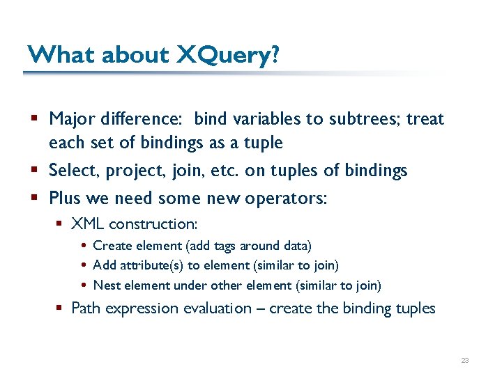
What about XQuery? § Major difference: bind variables to subtrees; treat each set of bindings as a tuple § Select, project, join, etc. on tuples of bindings § Plus we need some new operators: § XML construction: Create element (add tags around data) Add attribute(s) to element (similar to join) Nest element under other element (similar to join) § Path expression evaluation – create the binding tuples 23

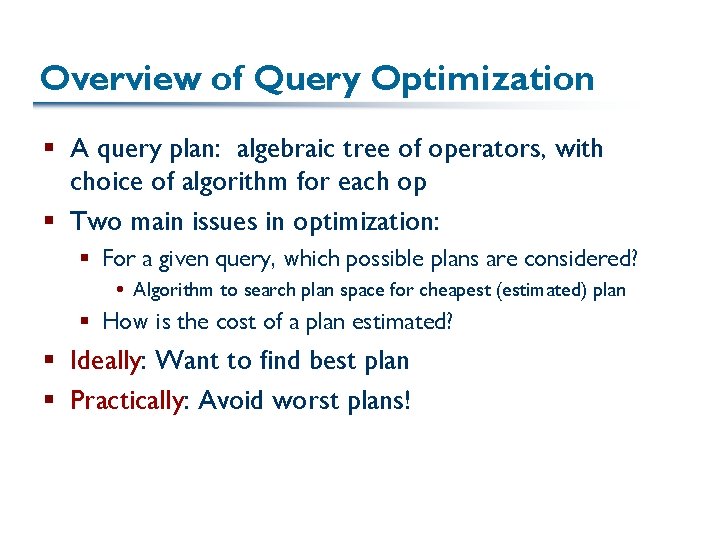
Overview of Query Optimization § A query plan: algebraic tree of operators, with choice of algorithm for each op § Two main issues in optimization: § For a given query, which possible plans are considered? Algorithm to search plan space for cheapest (estimated) plan § How is the cost of a plan estimated? § Ideally: Want to find best plan § Practically: Avoid worst plans!

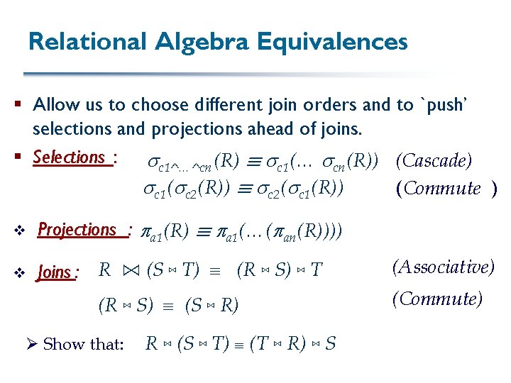
Relational Algebra Equivalences § Allow us to choose different join orders and to `push’ selections and projections ahead of joins. § Selections : c 1^…^cn (R) ´ c 1(… cn (R)) (Cascade) c 1( c 2(R)) ´ c 2( c 1(R)) (Commute ) v Projections : a 1 (R) ´ a 1 (…( an (R)))) v Joins : R ⋈ (S ⋈ T) (R ⋈ S) ⋈ T (R ⋈ S) (S ⋈ R) Ø Show that: R ⋈ (S ⋈ T) (T ⋈ R) ⋈ S (Associative) (Commute)

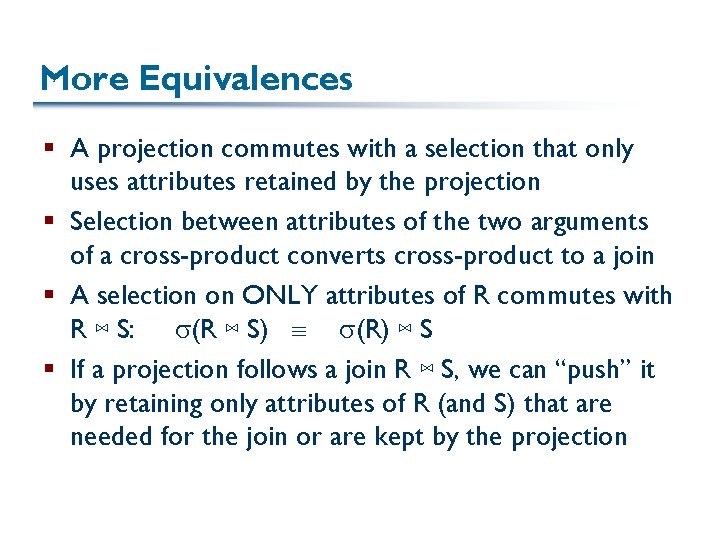
More Equivalences § A projection commutes with a selection that only uses attributes retained by the projection § Selection between attributes of the two arguments of a cross-product converts cross-product to a join § A selection on ONLY attributes of R commutes with R ⋈ S: (R ⋈ S) (R) ⋈ S § If a projection follows a join R ⋈ S, we can “push” it by retaining only attributes of R (and S) that are needed for the join or are kept by the projection

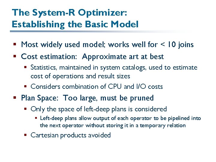
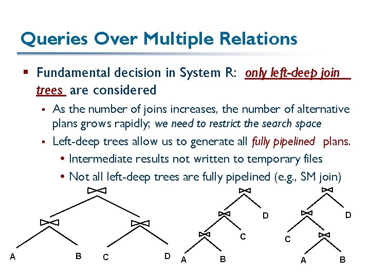
The System-R Optimizer: Establishing the Basic Model § Most widely used model; works well for < 10 joins § Cost estimation: Approximate art at best § Statistics, maintained in system catalogs, used to estimate cost of operations and result sizes § Considers combination of CPU and I/O costs § Plan Space: Too large, must be pruned § Only the space of left-deep plans is considered Left-deep plans allow output of each operator to be pipelined into the next operator without storing it in a temporary relation § Cartesian products avoided

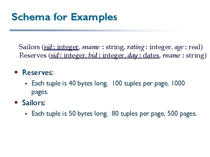
Schema for Examples Sailors (sid : integer, sname : string, rating : integer, age : real) Reserves (sid : integer, bid : integer, day : dates, rname : string) § Reserves: § Each tuple is 40 bytes long, 100 tuples per page, 1000 pages. § Sailors: § Each tuple is 50 bytes long, 80 tuples per page, 500 pages.

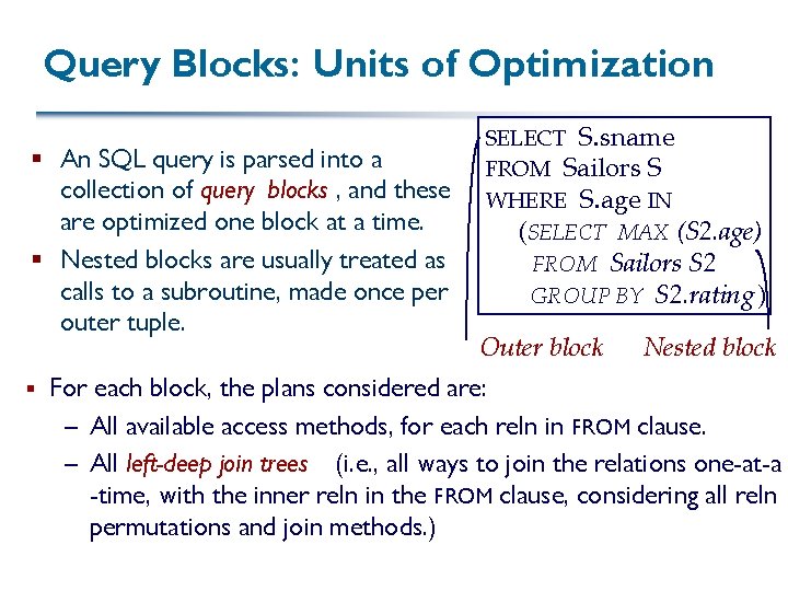
Query Blocks: Units of Optimization § An SQL query is parsed into a collection of query blocks , and these are optimized one block at a time. § Nested blocks are usually treated as calls to a subroutine, made once per outer tuple. § SELECT S. sname FROM Sailors S WHERE S. age IN (SELECT MAX (S 2. age) FROM Sailors S 2 GROUP BY S 2. rating ) Outer block Nested block For each block, the plans considered are: – All available access methods, for each reln in FROM clause. – All left-deep join trees (i. e. , all ways to join the relations one-at-a -time, with the inner reln in the FROM clause, considering all reln permutations and join methods. )

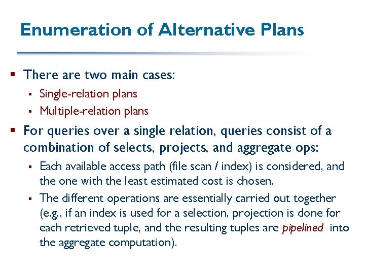
Enumeration of Alternative Plans § There are two main cases: § § Single-relation plans Multiple-relation plans § For queries over a single relation, queries consist of a combination of selects, projects, and aggregate ops: § § Each available access path (file scan / index) is considered, and the one with the least estimated cost is chosen. The different operations are essentially carried out together (e. g. , if an index is used for a selection, projection is done for each retrieved tuple, and the resulting tuples are pipelined into the aggregate computation).

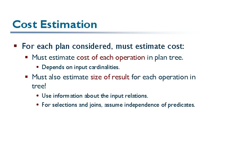
Cost Estimation § For each plan considered, must estimate cost: § Must estimate cost of each operation in plan tree. Depends on input cardinalities. § Must also estimate size of result for each operation in tree! Use information about the input relations. For selections and joins, assume independence of predicates.

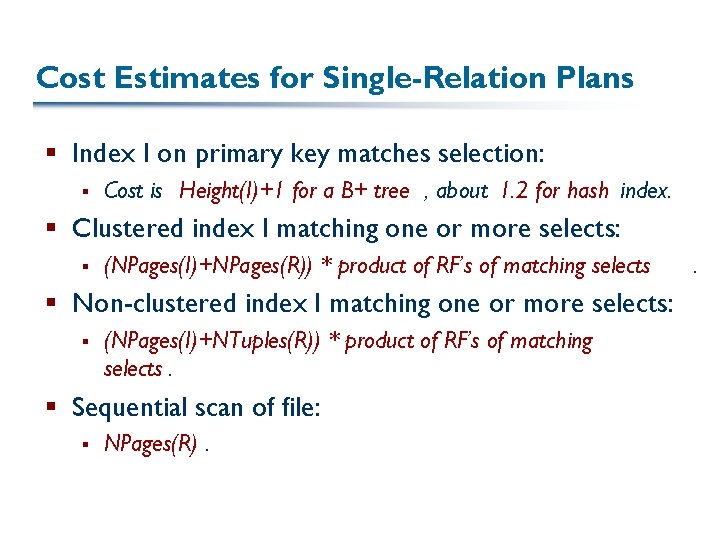
Cost Estimates for Single-Relation Plans § Index I on primary key matches selection: § Cost is Height(I)+1 for a B+ tree , about 1. 2 for hash index. § Clustered index I matching one or more selects: § (NPages(I)+NPages(R)) * product of RF’s of matching selects § Non-clustered index I matching one or more selects: § (NPages(I)+NTuples(R)) * product of RF’s of matching selects. § Sequential scan of file: § NPages(R). .

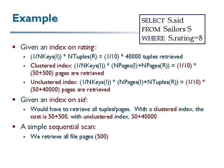
Example § Given an index on rating : § § § SELECT S. sid FROM Sailors S WHERE S. rating=8 (1/NKeys(I)) * NTuples(R) = (1/10) * 40000 tuples retrieved Clustered index: (1/NKeys(I)) * (NPages(I)+NPages(R)) = (1/10) * (50+500) pages are retrieved Unclustered index: (1/NKeys(I)) * (NPages(I)+NTuples(R)) = (1/10) * (50+40000) pages are retrieved § Given an index on sid : § Would have to retrieve all tuples/pages. With a clustered index, the cost is 50+500, with unclustered index, 50+40000 § A simple sequential scan: § We retrieve all file pages (500)

Queries Over Multiple Relations § Fundamental decision in System R: only left-deep join trees are considered § § As the number of joins increases, the number of alternative plans grows rapidly; we need to restrict the search space Left-deep trees allow us to generate all fully pipelined plans. Intermediate results not written to temporary files Not all left-deep trees are fully pipelined (e. g. , SM join) D D C A B C D A B C A B

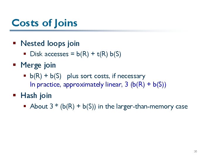
Costs of Joins § Nested loops join § Disk accesses = b(R) + t(R) b(S) § Merge join § b(R) + b(S) plus sort costs, if necessary In practice, approximately linear, 3 (b(R) + b(S)) § Hash join § About 3 * (b(R) + b(S)) in the larger-than-memory case 35