Purchasing Power Parities of Currencies and Real Expenditures

Purchasing Power Parities of Currencies and Real Expenditures – The International Comparison Program (ICP) D. S. Prasada Rao The University of Queensland 1

2

3

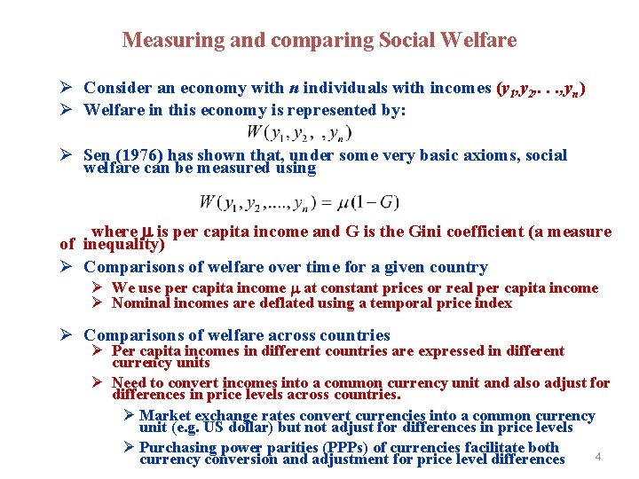
Measuring and comparing Social Welfare Ø Consider an economy with n individuals with incomes (y 1, y 2, . . . , yn) Ø Welfare in this economy is represented by: Ø Sen (1976) has shown that, under some very basic axioms, social welfare can be measured using where is per capita income and G is the Gini coefficient (a measure of inequality) Ø Comparisons of welfare over time for a given country Ø We use per capita income at constant prices or real per capita income Ø Nominal incomes are deflated using a temporal price index Ø Comparisons of welfare across countries Ø Per capita incomes in different countries are expressed in different currency units Ø Need to convert incomes into a common currency unit and also adjust for differences in price levels across countries. Ø Market exchange rates convert currencies into a common currency unit (e. g. US dollar) but not adjust for differences in price levels Ø Purchasing power parities (PPPs) of currencies facilitate both 4 currency conversion and adjustment for price level differences

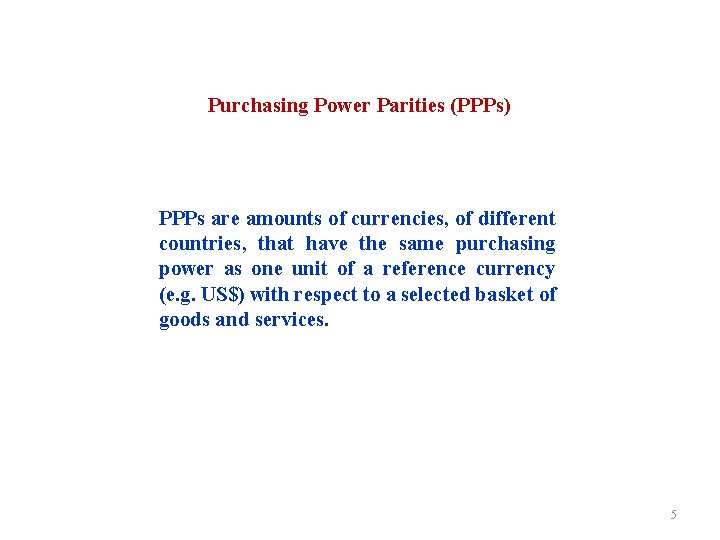
Purchasing Power Parities (PPPs) PPPs are amounts of currencies, of different countries, that have the same purchasing power as one unit of a reference currency (e. g. US$) with respect to a selected basket of goods and services. 5

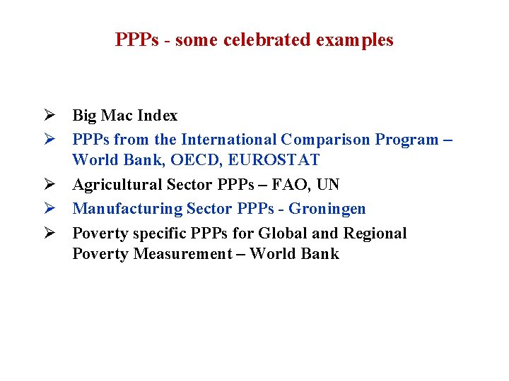
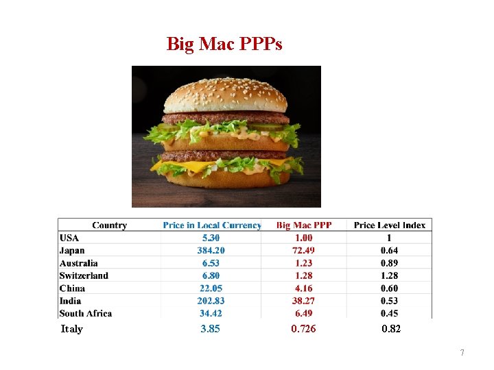
PPPs - some celebrated examples Ø Big Mac Index Ø PPPs from the International Comparison Program – World Bank, OECD, EUROSTAT Ø Agricultural Sector PPPs – FAO, UN Ø Manufacturing Sector PPPs - Groningen Ø Poverty specific PPPs for Global and Regional Poverty Measurement – World Bank

Big Mac PPPs Italy 3. 85 0. 726 0. 82 7

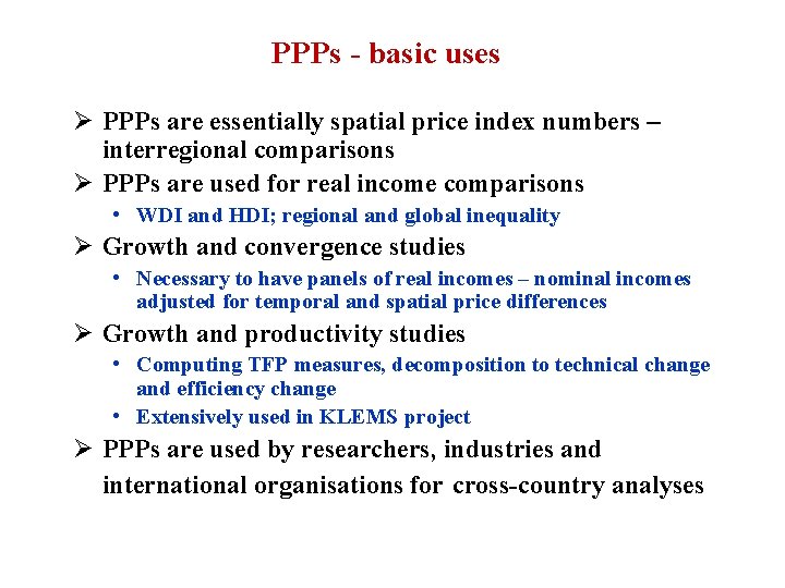
PPPs - basic uses Ø PPPs are essentially spatial price index numbers – interregional comparisons Ø PPPs are used for real income comparisons • WDI and HDI; regional and global inequality Ø Growth and convergence studies • Necessary to have panels of real incomes – nominal incomes adjusted for temporal and spatial price differences Ø Growth and productivity studies • Computing TFP measures, decomposition to technical change and efficiency change • Extensively used in KLEMS project Ø PPPs are used by researchers, industries and international organisations for cross-country analyses

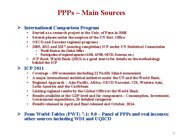
PPPs – Main Sources Ø International Comparison Program • • Started as a research project at the Univ. of Penn in 1968 Several phases under the auspices of the UN Stat. Office OECD and Eurostat regional programs 2005, 2011 and 2017 (nearing completion) ICP under UN Statistical Commission • • • World Bank as the Global Office Participation of regional agencies (ADB, AFDB, OECD, Eurostat, etc. ) ICP Book, World Bank (2013) is a good source for details on the methodology behind the ICP Ø ICP 2011 • • • Coverage – 199 economies (including 22 Pacific Island economies) A major international statistical initiative under the UN and the World Bank. Regional Approach – Asia-Pacific, Africa, OECD-Eurostat, CIS, Western Asia, Latin America and the Caribbean Linking regional results by the Global Office at the World Bank Results available at the GDP level and for components – Consumption, Investment, Government expenditure, 26 detailed categories Results released in April and final released end October, 2014. Ø Penn World Tables (PWT) 7. 1; 9. 0 – Panel of PPPs and real incomes; other sources including WDI and UQICD 9

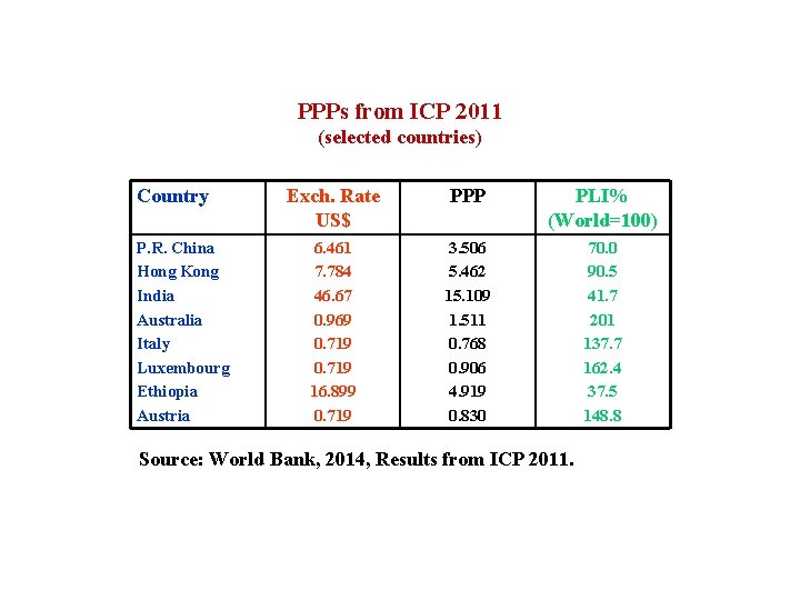
PPPs from ICP 2011 (selected countries) Country P. R. China Hong Kong India Australia Italy Luxembourg Ethiopia Austria Exch. Rate US$ PPP PLI% (World=100) 6. 461 7. 784 46. 67 0. 969 0. 719 16. 899 0. 719 3. 506 5. 462 15. 109 1. 511 0. 768 0. 906 4. 919 0. 830 70. 0 90. 5 41. 7 201 137. 7 162. 4 37. 5 148. 8 Source: World Bank, 2014, Results from ICP 2011.

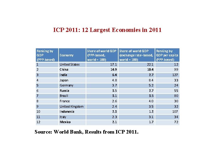
ICP 2011: 12 Largest Economies in 2011 Ranking by GDP (PPP-based) 1 2 3 4 5 6 7 8 9 10 11 12 Economy United States China India Japan Germany Russia Brazil France United Kingdom Indonesia Italy Mexico Share of world GDP Ranking by (PPP-based, (exchange rate–based, GDP per capita world = 100) (PPP-based) 17. 1 22. 1 12 14. 9 10. 4 99 6. 4 2. 7 127 4. 8 8. 4 33 3. 7 5. 2 24 3. 5 2. 7 55 3. 1 3. 5 80 2. 6 4. 0 30 2. 4 3. 5 32 2. 3 1. 2 107 2. 3 3. 1 34 2. 1 1. 7 72 Source: World Bank, Results from ICP 2011.

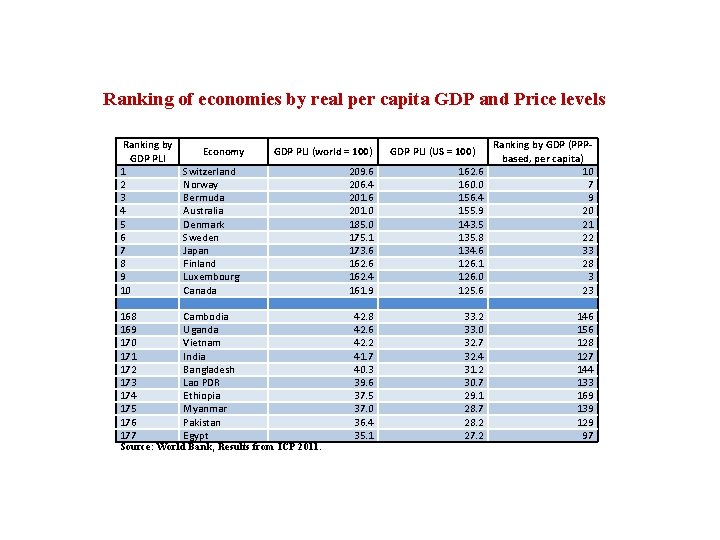
Ranking of economies by real per capita GDP and Price levels Ranking by GDP PLI 1 2 3 4 5 6 7 8 9 10 Economy 209. 6 206. 4 201. 6 201. 0 185. 0 175. 1 173. 6 162. 4 161. 9 162. 6 160. 0 156. 4 155. 9 143. 5 135. 8 134. 6 126. 1 126. 0 125. 6 Ranking by GDP (PPPbased, per capita) 10 7 9 20 21 22 33 28 3 23 42. 8 42. 6 42. 2 41. 7 40. 3 39. 6 37. 5 37. 0 36. 4 35. 1 33. 2 33. 0 32. 7 32. 4 31. 2 30. 7 29. 1 28. 7 28. 2 27. 2 146 156 128 127 144 133 169 139 129 97 GDP PLI (world = 100) Switzerland Norway Bermuda Australia Denmark Sweden Japan Finland Luxembourg Canada 168 Cambodia 169 Uganda 170 Vietnam 171 India 172 Bangladesh 173 Lao PDR 174 Ethiopia 175 Myanmar 176 Pakistan 177 Egypt Source: World Bank, Results from ICP 2011. GDP PLI (US = 100)

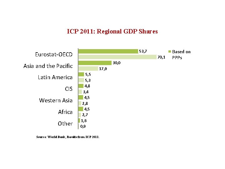
ICP 2011: Regional GDP Shares 53, 7 Eurostat-OECD 70, 1 30, 0 Asia and the Pacific Latin America CIS Western Asia Africa Other 17, 9 5, 5 5, 3 4, 8 3, 4 4, 5 2, 8 4, 5 2, 7 1, 6 0, 9 Source: World Bank, Results from ICP 2011. Based on PPPs

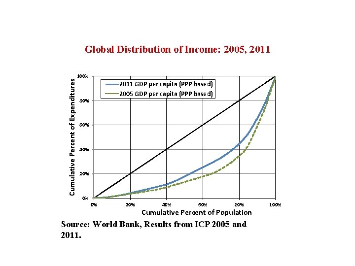
Cumulative Percent of Expenditures Global Distribution of Income: 2005, 2011 100% 2011 GDP per capita (PPP based) 2005 GDP per capita (PPP based) 80% 60% 40% 20% 0% 0% 20% 40% 60% 80% Cumulative Percent of Population Source: World Bank, Results from ICP 2005 and 2011. 100%

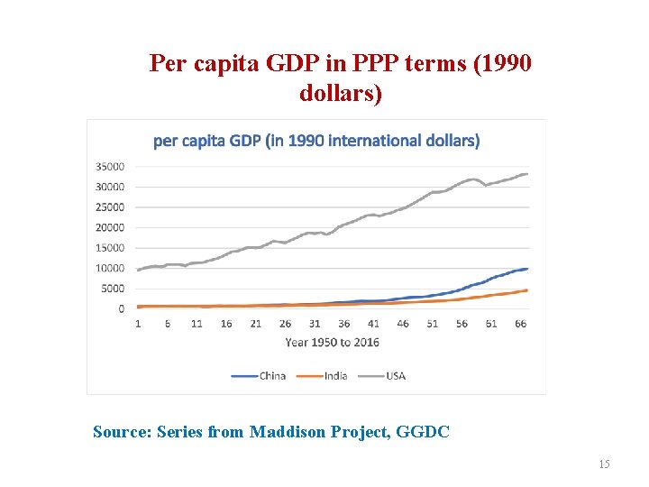
Per capita GDP in PPP terms (1990 dollars) Source: Series from Maddison Project, GGDC 15

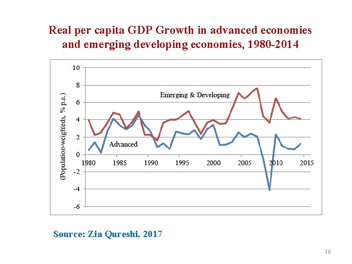
Real per capita GDP Growth in advanced economies and emerging developing economies, 1980 -2014 Source: Zia Qureshi, 2017 16

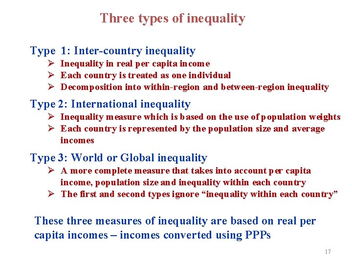
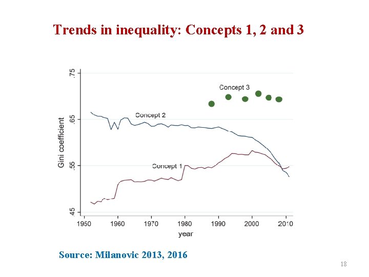
Three types of inequality Type 1: Inter-country inequality Ø Inequality in real per capita income Ø Each country is treated as one individual Ø Decomposition into within-region and between-region inequality Type 2: International inequality Ø Inequality measure which is based on the use of population weights Ø Each country is represented by the population size and average incomes Type 3: World or Global inequality Ø A more complete measure that takes into account per capita income, population size and inequality within each country Ø The first and second types ignore “inequality within each country” These three measures of inequality are based on real per capita incomes – incomes converted using PPPs 17

Trends in inequality: Concepts 1, 2 and 3 Source: Milanovic 2013, 2016 18

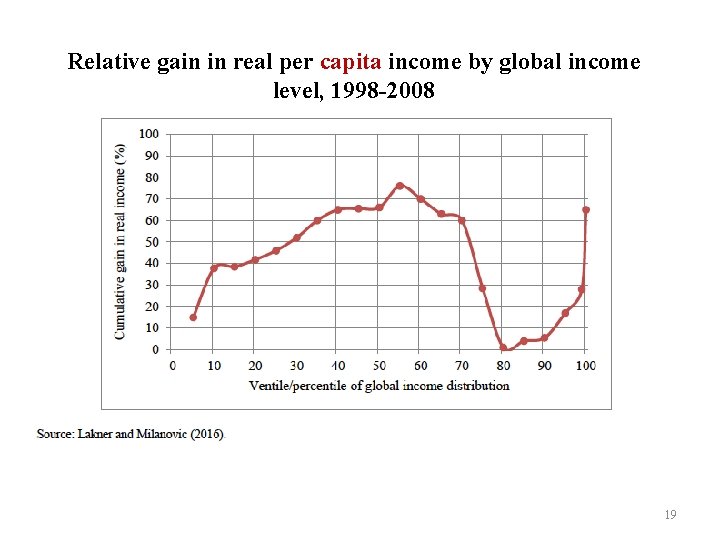
Relative gain in real per capita income by global income level, 1998 -2008 19

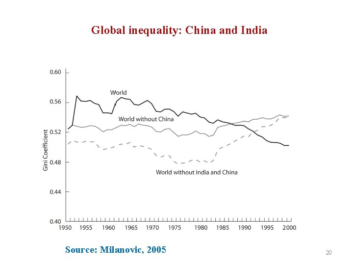
Global inequality: China and India Source: Milanovic, 2005 20

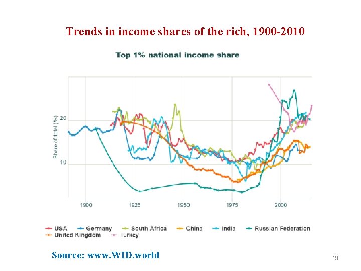
Trends in income shares of the rich, 1900 -2010 Source: www. WID. world 21

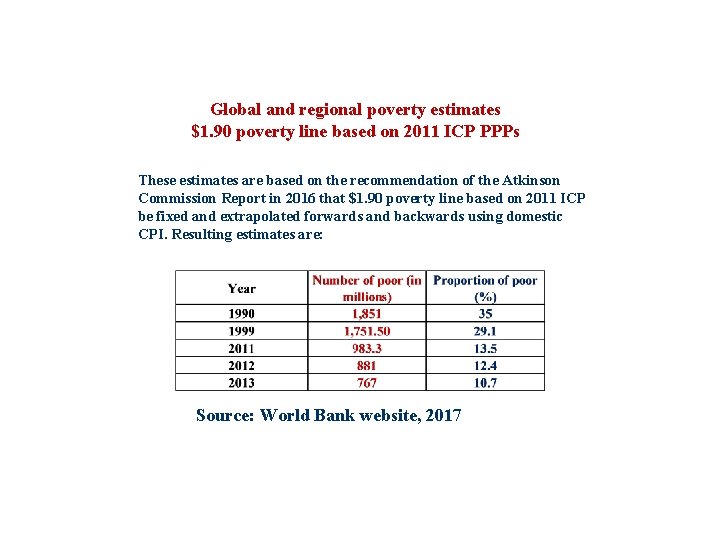
Global and regional poverty estimates $1. 90 poverty line based on 2011 ICP PPPs These estimates are based on the recommendation of the Atkinson Commission Report in 2016 that $1. 90 poverty line based on 2011 ICP be fixed and extrapolated forwards and backwards using domestic CPI. Resulting estimates are: Source: World Bank website, 2017

PPP Measurement and the International Comparison Program

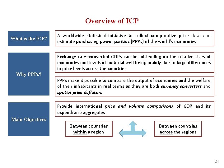
Overview of ICP What is the ICP? A worldwide statistical initiative to collect comparative price data and estimate purchasing power parities (PPPs) of the world’s economies Exchange rate–converted GDPs can be misleading on the relative sizes of economies and levels of material well-being mainly due to large differences in price levels across the countries Why PPPs? PPPs make it possible to compare the output of economies and the welfare of their inhabitants in real terms as they are both currency converters and spatial price deflators Provide international price and volume comparisons of GDP and its expenditure aggregates Main Objectives Between countries within a region Between countries across the regions 24

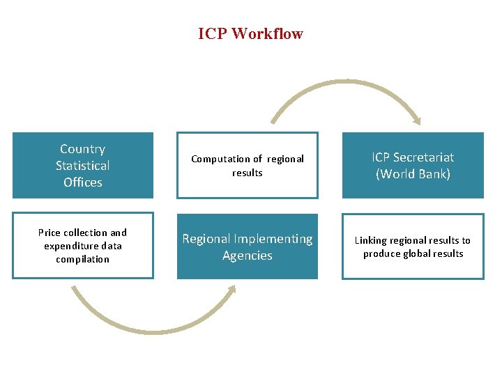
ICP Workflow Country Statistical Offices Computation of regional results ICP Secretariat (World Bank) Price collection and expenditure data compilation Regional Implementing Agencies Linking regional results to produce global results

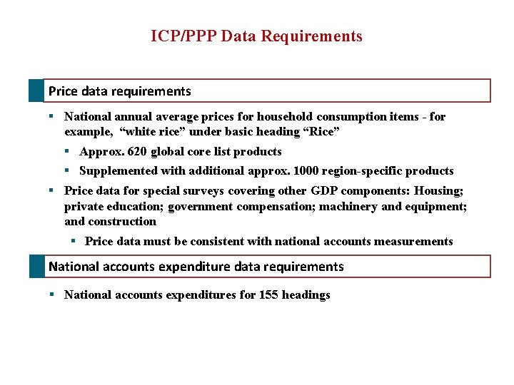
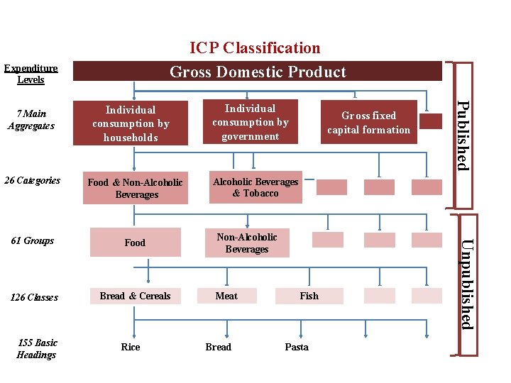
ICP/PPP Data Requirements Price data requirements § National annual average prices for household consumption items - for example, “white rice” under basic heading “Rice” § Approx. 620 global core list products § Supplemented with additional approx. 1000 region-specific products § Price data for special surveys covering other GDP components: Housing; private education; government compensation; machinery and equipment; and construction § Price data must be consistent with national accounts measurements National accounts expenditure data requirements § National accounts expenditures for 155 headings

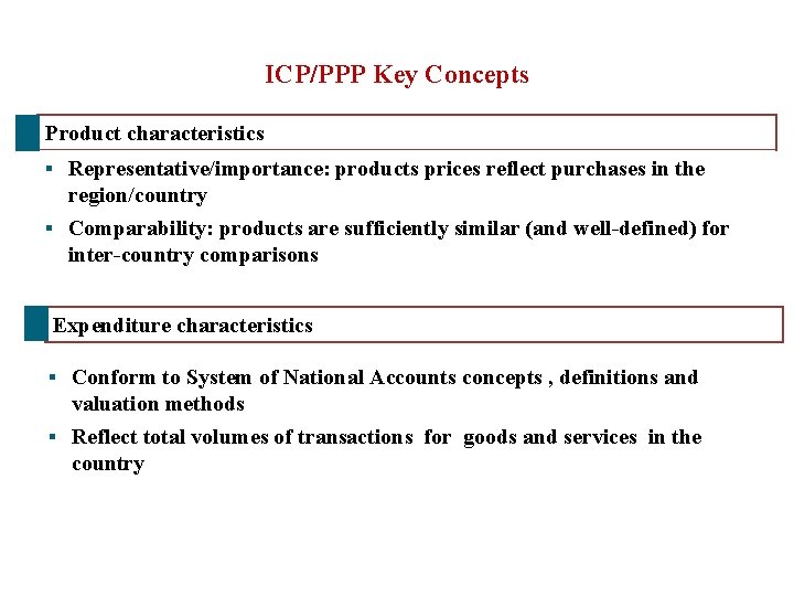
ICP/PPP Key Concepts Product characteristics § Representative/importance: products prices reflect purchases in the region/country § Comparability: products are sufficiently similar (and well-defined) for inter-country comparisons Expenditure characteristics § Conform to System of National Accounts concepts , definitions and valuation methods § Reflect total volumes of transactions for goods and services in the country

ICP Classification Gross Domestic Product Expenditure Levels Individual consumption by households Food & Non-Alcoholic Beverages 61 Groups Food 126 Classes Bread & Cereals 155 Basic Headings Rice Gross fixed capital formation Alcoholic Beverages & Tobacco Non-Alcoholic Beverages Meat Bread Fish Pasta Unpublished 26 Categories Individual consumption by government Published 7 Main Aggregates

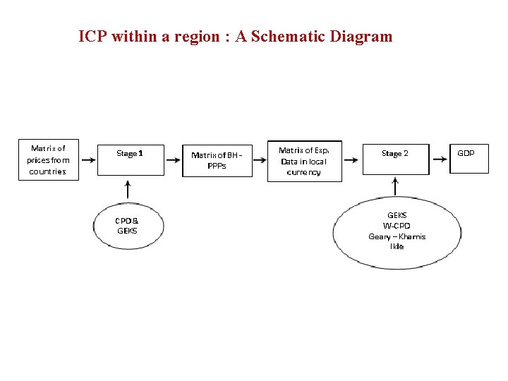
ICP within a region : A Schematic Diagram

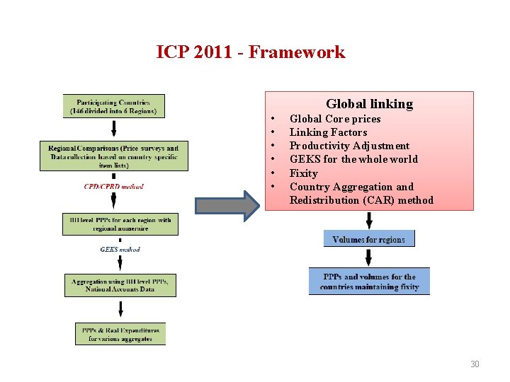
ICP 2011 - Framework Global linking • • • Global Core prices Linking Factors Productivity Adjustment GEKS for the whole world Fixity Country Aggregation and Redistribution (CAR) method 30

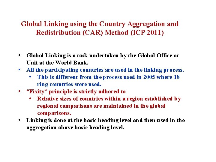
Global Linking using the Country Aggregation and Redistribution (CAR) Method (ICP 2011) • Global Linking is a task undertaken by the Global Office or Unit at the World Bank. • All the participating countries are used in the linking process. • This is different from the process used in 2005 where 18 ring countries were used. • “Fixity” principle is strictly adhered to • Relative sizes of countries within a region established by regional comparisons are maintained in the global comparisons. • Linking is done at the basic heading level and then used in the aggregation above basic heading level.

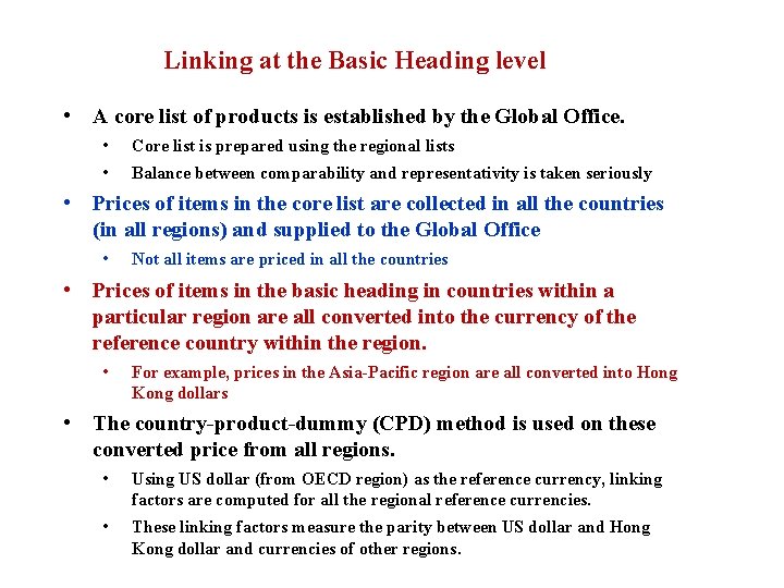
Linking at the Basic Heading level • A core list of products is established by the Global Office. • Core list is prepared using the regional lists • Balance between comparability and representativity is taken seriously • Prices of items in the core list are collected in all the countries (in all regions) and supplied to the Global Office • Not all items are priced in all the countries • Prices of items in the basic heading in countries within a particular region are all converted into the currency of the reference country within the region. • For example, prices in the Asia-Pacific region are all converted into Hong Kong dollars • The country-product-dummy (CPD) method is used on these converted price from all regions. • Using US dollar (from OECD region) as the reference currency, linking factors are computed for all the regional reference currencies. • These linking factors measure the parity between US dollar and Hong Kong dollar and currencies of other regions.

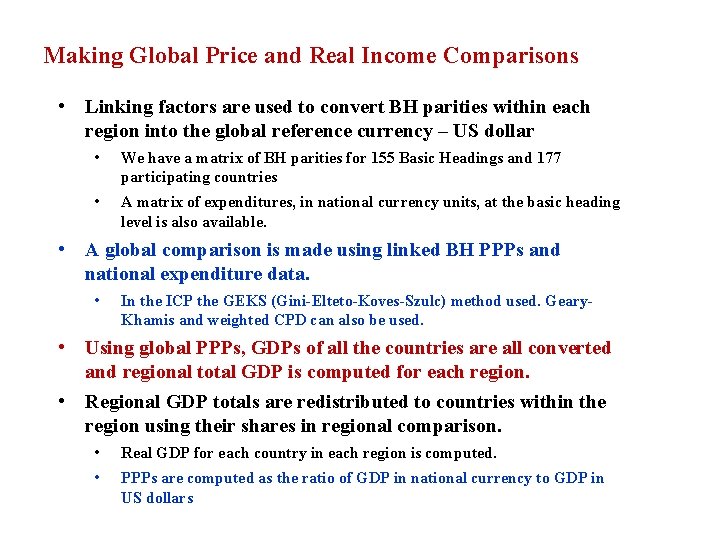
Making Global Price and Real Income Comparisons • Linking factors are used to convert BH parities within each region into the global reference currency – US dollar • We have a matrix of BH parities for 155 Basic Headings and 177 participating countries • A matrix of expenditures, in national currency units, at the basic heading level is also available. • A global comparison is made using linked BH PPPs and national expenditure data. • In the ICP the GEKS (Gini-Elteto-Koves-Szulc) method used. Geary. Khamis and weighted CPD can also be used. • Using global PPPs, GDPs of all the countries are all converted and regional total GDP is computed for each region. • Regional GDP totals are redistributed to countries within the region using their shares in regional comparison. • Real GDP for each country in each region is computed. • PPPs are computed as the ratio of GDP in national currency to GDP in US dollars

Index Number Methods for computing PPPs

Multilateral Comparisons - Data

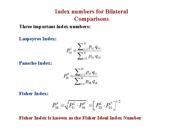
Index numbers for Bilateral Comparisons Three important index numbers: Laspeyres Index: Paasche Index: Fisher Index is known as the Fisher Ideal Index Number

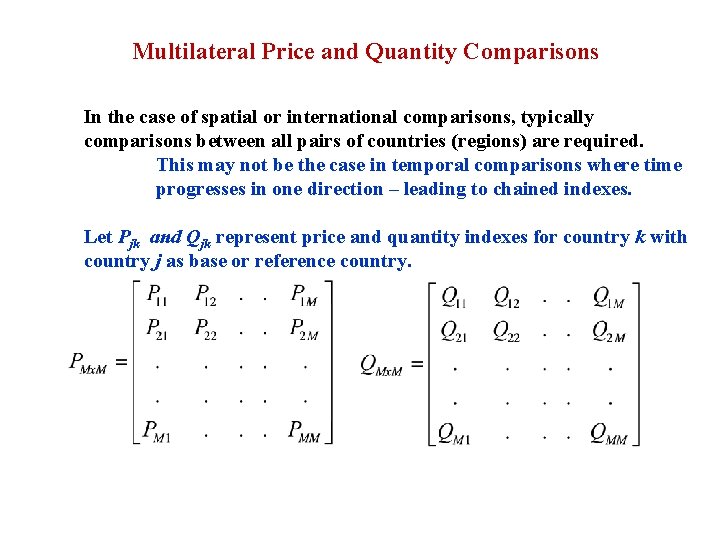
Multilateral Price and Quantity Comparisons In the case of spatial or international comparisons, typically comparisons between all pairs of countries (regions) are required. This may not be the case in temporal comparisons where time progresses in one direction – leading to chained indexes. Let Pjk and Qjk represent price and quantity indexes for country k with country j as base or reference country.

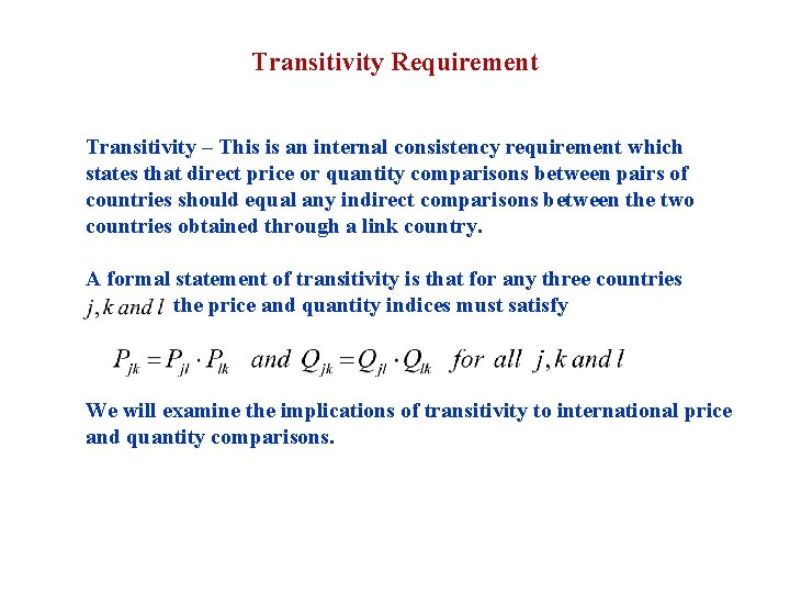
Transitivity Requirement Transitivity – This is an internal consistency requirement which states that direct price or quantity comparisons between pairs of countries should equal any indirect comparisons between the two countries obtained through a link country. A formal statement of transitivity is that for any three countries the price and quantity indices must satisfy We will examine the implications of transitivity to international price and quantity comparisons.

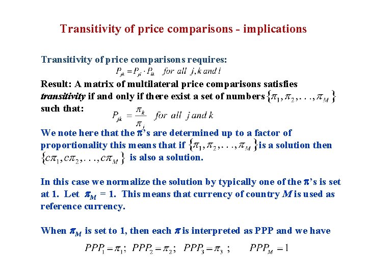
Transitivity of price comparisons - implications Transitivity of price comparisons requires: Result: A matrix of multilateral price comparisons satisfies transitivity if and only if there exist a set of numbers such that: We note here that the ’s are determined up to a factor of proportionality this means that if is a solution then is also a solution. In this case we normalize the solution by typically one of the ’s is set at 1. Let M = 1. This means that currency of country M is used as reference currency. When M is set to 1, then each is interpreted as PPP and we have

Gini-Elteto-Koves-Szulc (GEKS) and weighted GEKS methods for aggregation below and above basic heading level

Gini-Elteto-Koves-Szulc Method • This method was previously known as the Elteto-Koves. Szulc (EKS) method which proposed in 1964. • The EKS method was the preferred method of aggregation below and above the basic heading level in the EU region. • A decade ago it was discovered that Gini proposed a similar method in 1924 and also mentioned in his work in 1931, “On the Circular Test of Index Numbers” published in the International Review of Statistics. • It has since then been referred to as the GEKS method • Since the 2005 round of the ICP, GEKS has been the recommended method for aggregation above the basic heading level. • It is only recently a generalization known as the weighted GEKS has been proposed and discussed.

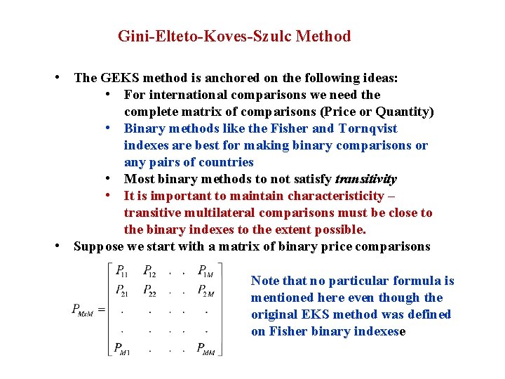
Gini-Elteto-Koves-Szulc Method • The GEKS method is anchored on the following ideas: • For international comparisons we need the complete matrix of comparisons (Price or Quantity) • Binary methods like the Fisher and Tornqvist indexes are best for making binary comparisons or any pairs of countries • Most binary methods to not satisfy transitivity • It is important to maintain characteristicity – transitive multilateral comparisons must be close to the binary indexes to the extent possible. • Suppose we start with a matrix of binary price comparisons Note that no particular formula is mentioned here even though the original EKS method was defined on Fisher binary indexese

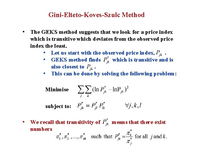
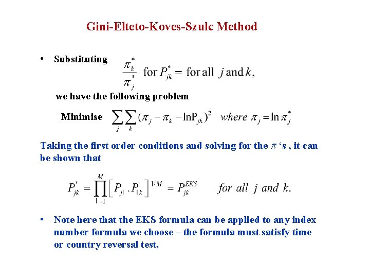
Gini-Elteto-Koves-Szulc Method • The GEKS method suggests that we look for a price index which is transitive which deviates from the observed price index the least. • Let us start with the observed price index, . • GEKS method finds which is transitive and is also closest to. • This can be done by solving the following problem: Minimise subject to: • We recall that transitivity of numbers means that there exist

Gini-Elteto-Koves-Szulc Method • Substituting we have the following problem Minimise Taking the first order conditions and solving for the ‘s , it can be shown that • Note here that the EKS formula can be applied to any index number formula we choose – the formula must satisfy time or country reversal test.

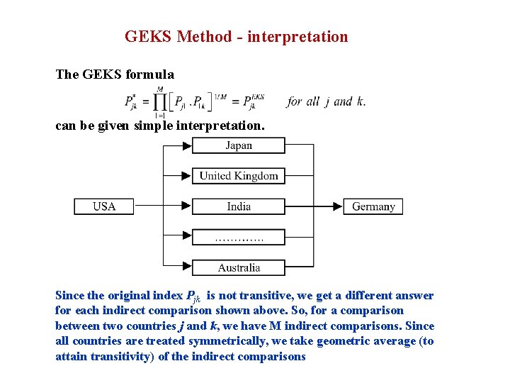
GEKS Method - interpretation The GEKS formula can be given simple interpretation. Since the original index Pjk is not transitive, we get a different answer for each indirect comparison shown above. So, for a comparison between two countries j and k, we have M indirect comparisons. Since all countries are treated symmetrically, we take geometric average (to attain transitivity) of the indirect comparisons

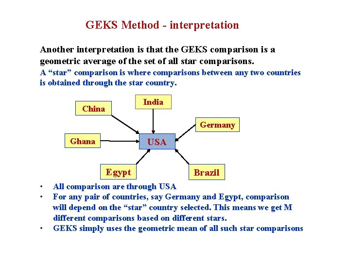
GEKS Method - interpretation Another interpretation is that the GEKS comparison is a geometric average of the set of all star comparisons. A “star” comparison is where comparisons between any two countries is obtained through the star country. India China Germany Ghana USA Egypt • • • Brazil All comparison are through USA For any pair of countries, say Germany and Egypt, comparison will depend on the “star” country selected. This means we get M different comparisons based on different stars. GEKS simply uses the geometric mean of all such star comparisons

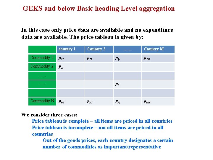
GEKS and below Basic heading Level aggregation In this case only price data are available and no expenditure data are available. The price tableau is given by: country 1 Country 2 Commodity 1 p 12 Commodity 2 p 21 …… p 1 j Country M p 1 M …… …… Commodity N pij p. N 1 p. N 2 p. Nj p. NM We consider three cases: Price tableau is complete – all items are priced in all countries Price tableau is incomplete – not all items are priced in all countries Out of the goods prices, each country designates a certain number of commodities as important/representative

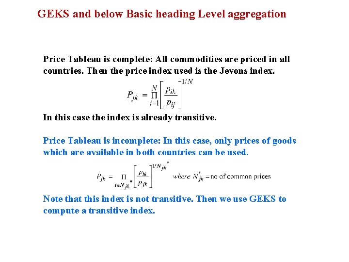
GEKS and below Basic heading Level aggregation Price Tableau is complete: All commodities are priced in all countries. Then the price index used is the Jevons index. In this case the index is already transitive. Price Tableau is incomplete: In this case, only prices of goods which are available in both countries can be used. Note that this index is not transitive. Then we use GEKS to compute a transitive index.

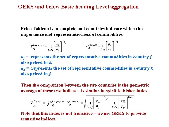
GEKS and below Basic heading Level aggregation Price Tableau is incomplete and countries indicate which the importance and representativeness of commodities. nj = represents the set of representative commodities in country j also priced in k. nk = represents the set of representative commodities in country k also priced in j. Then the comparison between the two countries is the geometric average of these two indices – is similar in spirit to Fisher index Note that this index is not transitive – we use GEKS to provide transitive indices.

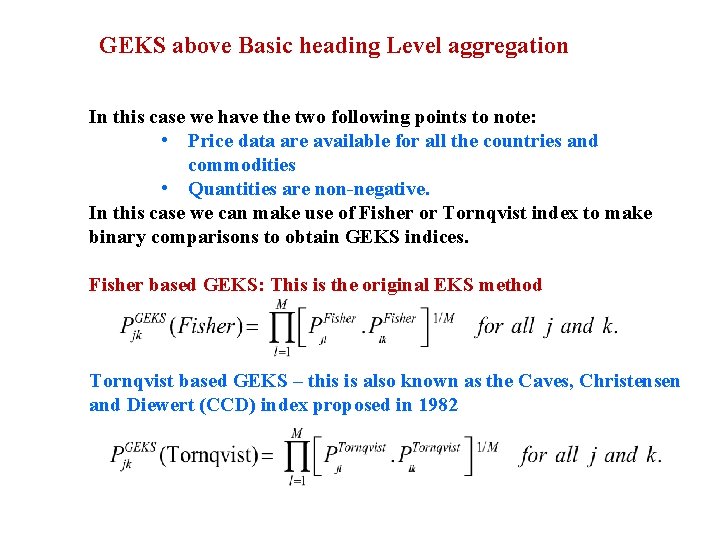
GEKS above Basic heading Level aggregation In this case we have the two following points to note: • Price data are available for all the countries and commodities • Quantities are non-negative. In this case we can make use of Fisher or Tornqvist index to make binary comparisons to obtain GEKS indices. Fisher based GEKS: This is the original EKS method Tornqvist based GEKS – this is also known as the Caves, Christensen and Diewert (CCD) index proposed in 1982

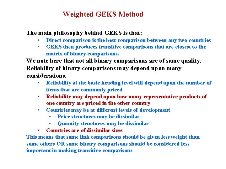
Weighted GEKS Method The main philosophy behind GEKS is that: • • Direct comparison is the best comparison between any two countries GEKS then produces transitive comparisons that are closest to the matrix of binary comparisons. We note here that not all binary comparisons are of same quality. Reliability of binary comparisons may depend upon many considerations. • Reliability at the basic heading level will depend upon the number of items that are commonly priced • Reliability may depend upon how many representative products of one country are priced in the other country • Countries may be at different levels of development • Price structures may be dissimilar • Quantity structures may be dissimilar • Countries are of dissimilar sizes This means that some link comparisons should be given less weight than some others OR some binary comparisons should be considered less important in making transitive comparisons

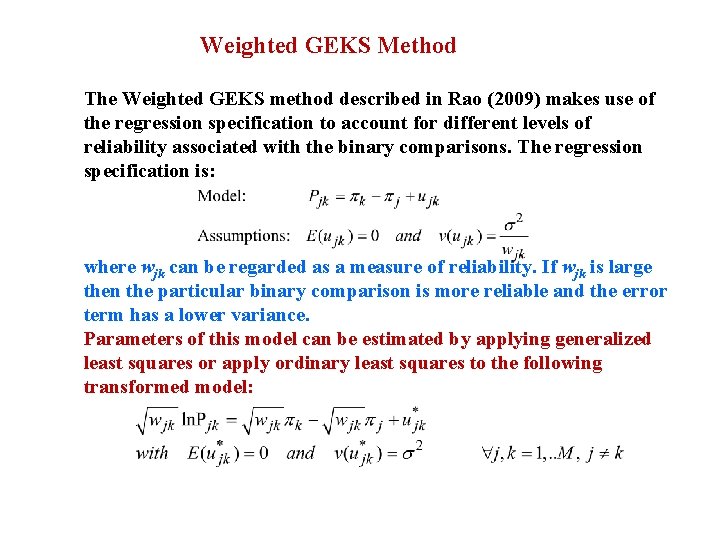
Weighted GEKS Method The Weighted GEKS method described in Rao (2009) makes use of the regression specification to account for different levels of reliability associated with the binary comparisons. The regression specification is: where wjk can be regarded as a measure of reliability. If wjk is large then the particular binary comparison is more reliable and the error term has a lower variance. Parameters of this model can be estimated by applying generalized least squares or apply ordinary least squares to the following transformed model:

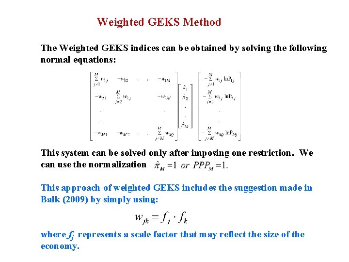
Weighted GEKS Method The Weighted GEKS indices can be obtained by solving the following normal equations: This system can be solved only after imposing one restriction. We can use the normalization This approach of weighted GEKS includes the suggestion made in Balk (2009) by simply using: where fj represents a scale factor that may reflect the size of the economy.

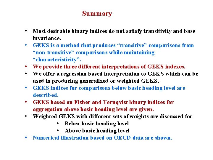
Summary • Most desirable binary indices do not satisfy transitivity and base invariance. • GEKS is a method that produces “transitive” comparisons from “non-transitive” comparisons while maintaining “characteristicity”. • We provide three different interpretations of GEKS indexes. • We offer a regression based interpretation to GEKS which can be used in producing generalized or weighted GEKS. • GEKS indices for comparisons below basic heading level are described. • GEKS based on Fisher and Tornqvist binary indices for aggregation above basic heading level are given. • Weighted GEKS with different sets of weights are discussed for • Below basic heading level • Above basic heading level • Numerical illustration based on OECD data are shown.

The Country-Product-Dummy (CPD) Method

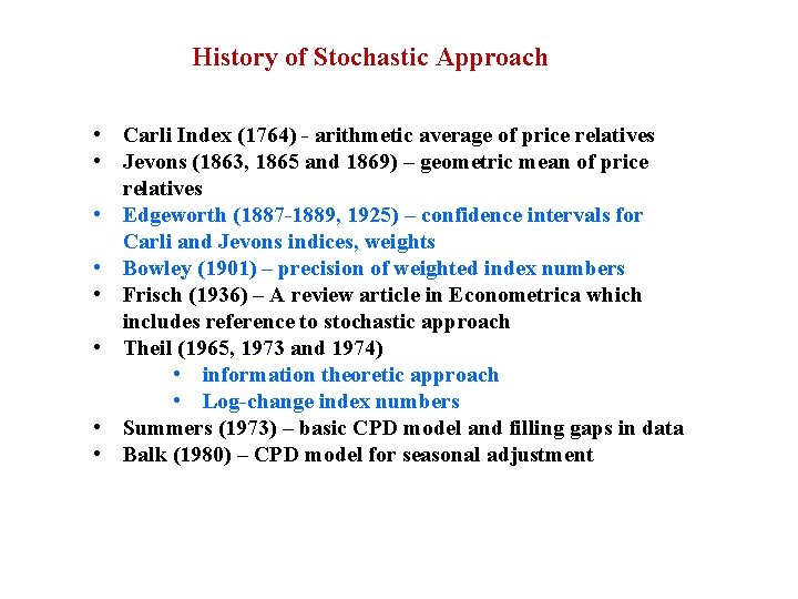
History of Stochastic Approach • Carli Index (1764) - arithmetic average of price relatives • Jevons (1863, 1865 and 1869) – geometric mean of price relatives • Edgeworth (1887 -1889, 1925) – confidence intervals for Carli and Jevons indices, weights • Bowley (1901) – precision of weighted index numbers • Frisch (1936) – A review article in Econometrica which includes reference to stochastic approach • Theil (1965, 1973 and 1974) • information theoretic approach • Log-change index numbers • Summers (1973) – basic CPD model and filling gaps in data • Balk (1980) – CPD model for seasonal adjustment

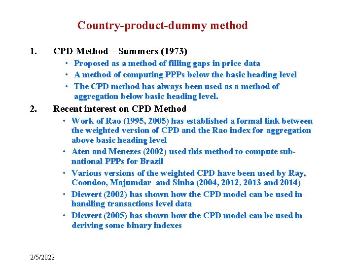
Country-product-dummy method 1. CPD Method – Summers (1973) • Proposed as a method of filling gaps in price data • A method of computing PPPs below the basic heading level • The CPD method has always been used as a method of aggregation below basic heading level. 2. Recent interest on CPD Method • Work of Rao (1995, 2005) has established a formal link between the weighted version of CPD and the Rao index for aggregation above basic heading level • Aten and Menezes (2002) used this method to compute subnational PPPs for Brazil • Various versions of the weighted CPD have been used by Ray, Coondoo, Majumdar and Sinha (2004, 2012, 2013 and 2014) • Diewert (2002) has shown how the CPD model can be used in handling transactions level data • Diewert (2005) has shown how the CPD model can be used in deriving some binary indexes 2/5/2022

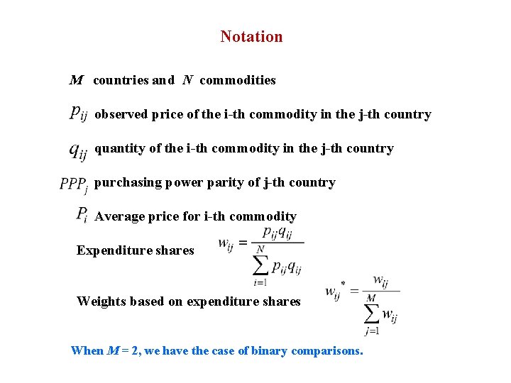
Notation M countries and N commodities observed price of the i-th commodity in the j-th country quantity of the i-th commodity in the j-th country purchasing power parity of j-th country Average price for i-th commodity Expenditure shares Weights based on expenditure shares When M = 2, we have the case of binary comparisons.

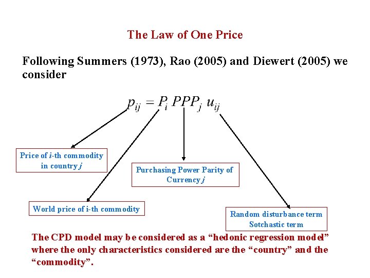
The Law of One Price Following Summers (1973), Rao (2005) and Diewert (2005) we consider Price of i-th commodity in country j Purchasing Power Parity of Currency j World price of i-th commodity Random disturbance term Sotchastic term The CPD model may be considered as a “hedonic regression model” where the only characteristics considered are the “country” and the “commodity”.

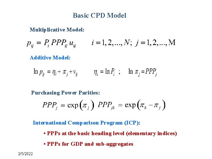
Basic CPD Model Multiplicative Model: Additive Model: Purchasing Power Parities: International Comparison Program (ICP): • PPPs at the basic heading level (elementary indices) • PPPs for GDP and sub-aggregates 2/5/2022

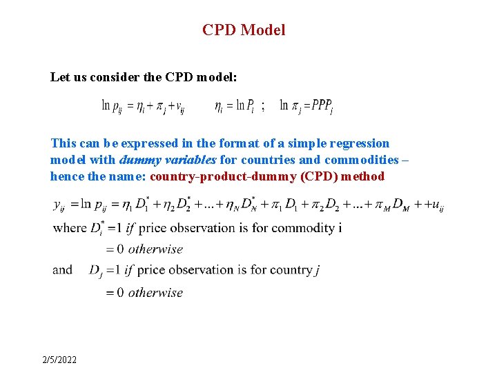
CPD Model Let us consider the CPD model: This can be expressed in the format of a simple regression model with dummy variables for countries and commodities – hence the name: country-product-dummy (CPD) method 2/5/2022

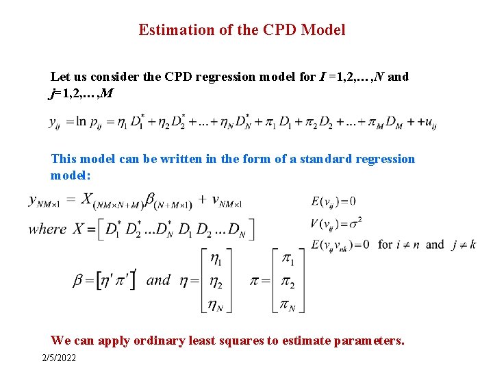
Estimation of the CPD Model Let us consider the CPD regression model for I =1, 2, …, N and j=1, 2, …, M This model can be written in the form of a standard regression model: We can apply ordinary least squares to estimate parameters. 2/5/2022

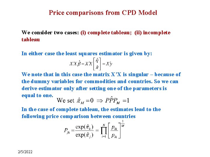
Price comparisons from CPD Model We consider two cases: (i) complete tableau; (ii) incomplete tableau In either case the least squares estimator is given by: We note that in this case the matrix X’X is singular – because of the dummy variables for commodities and countries. So we can derive estimator only after setting one of the parameters is equal to one. In the case of complete tableau, the estimates lead to the following price comparison between countries 2/5/2022

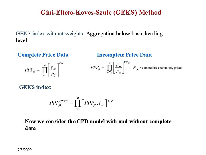
Gini-Elteto-Koves-Szulc (GEKS) Method GEKS index without weights: Aggregation below basic heading level Complete Price Data Incomplete Price Data GEKS index: Now we consider the CPD model with and without complete data 2/5/2022

CPD price comparisons - continued • Standard properties of least squares estimators hold for • Exp ( ) is not an unbiased estimator of PPPj • Under lognormality of residuals of the multiplicative model, it is possible to derive UMVUE of PPPj. • Estimated standard errors can be calculated for estimator of PPPj without any distributional assumptions • When price tableau is complete, standard errors of are the same for all c; however, they vary for estimators of PPP’s. • With complete price data, the CPD estimator of PPPs is identical to the GEKS PPPs – both methods give the same answer • When price tableau is incomplete, the CPD estimator makes use of all the information that is available. • If a commodity is priced in only country that information will not be used in the model 2/5/2022

CPD price comparisons - continued • If the disturbances in the original CPD model are log-normal, then the disturbances in the regression model, vij , are normally distributed. • This means that we can use standard t-tests and confidence intervals for the PPPs. • The regression approach minimizes the residual sum of squares: • In this case all the price observations are given equal weight. • However if there is additional information available on weights in the form of expenditure shares or importance then we can minimize weighted sum of squares • The current recommendation is to give weight 3 if the product is important and 1 if it is not important. Question is what weights to give? • We are currently using scanner data to determine weights for items that are considered important. 2/5/2022

CPD with incomplete price data • In ICP, countries within a region are all given a list of products with well specified product characteristics for purposes of price collection. • Price tableau is usually incomplete – can be quite sparse. • The CPD model can be applied to the incomplete price data provided data are not too sparse. • The paper states a few conditions under which the CPD regression model can provide estimates of all the parameters when one linear restriction is imposed. • A necessary and sufficient condition for the CPD model to work is that the “graph” associated with the price data is connected. • The extent of sparseness influences the standard errors. 2/5/2022

CPD with incomplete price data • Role of CPD as a filler of missing price data • Once the CPD model is estimated with available data, it can be used in filling gaps with predicted prices – original idea of Summers (1973). • Once the price tableau is complete after filling gaps, it is possible to use GEKS on the full data set. • Rao (2004) showed that the GEKS PPPs derived using CPD fillers are identical to the PPPs estimated from the CPD model on incomplete data. • This follows from the fact that the regression estimates do not change if we augment price tableau with predictions from the GCPD – no free lunch! • However, GEKS applied on incomplete data and GEKS applied to filled data differ – this means CPD is superior to GEKS 2/5/2022

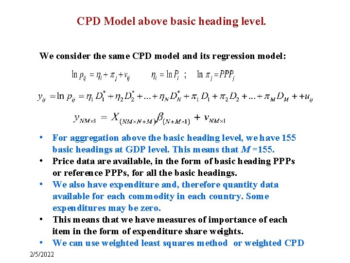
CPD Model above basic heading level. We consider the same CPD model and its regression model: • For aggregation above the basic heading level, we have 155 basic headings at GDP level. This means that M =155. • Price data are available, in the form of basic heading PPPs or reference PPPs, for all the basic headings. • We also have expenditure and, therefore quantity data available for each commodity in each country. Some expenditures may be zero. • This means that we have measures of importance of each item in the form of expenditure share weights. • We can use weighted least squares method or weighted CPD 2/5/2022

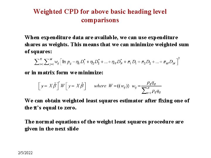
Weighted CPD for above basic heading level comparisons When expenditure data are available, we can use expenditure shares as weights. This means that we can minimize weighted sum of squares: or in matrix form we minimize: We can obtain weighted least squares estimator after fixing one of the ’s equal to zero. The normal equations of the weight least squares procedure are given in the next slide 2/5/2022

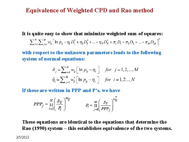
Equivalence of Weighted CPD and Rao method It is quite easy to show that minimize weighted sum of squares: with respect to the unknown parameters leads to the following system of normal equations: If these are written in PPP and P’s, we have These equations are identical to the equations that determine the Rao (1990) system – this establishes equivalence of the two systems. 2/5/2022

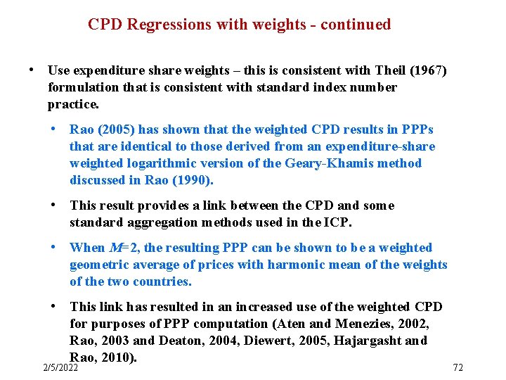
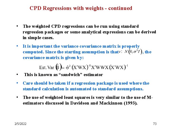
CPD Regressions with weights - continued • Use expenditure share weights – this is consistent with Theil (1967) formulation that is consistent with standard index number practice. • Rao (2005) has shown that the weighted CPD results in PPPs that are identical to those derived from an expenditure-share weighted logarithmic version of the Geary-Khamis method discussed in Rao (1990). • This result provides a link between the CPD and some standard aggregation methods used in the ICP. • When M=2, the resulting PPP can be shown to be a weighted geometric average of prices with harmonic mean of the weights of the two countries. • This link has resulted in an increased use of the weighted CPD for purposes of PPP computation (Aten and Menezies, 2002, Rao, 2003 and Deaton, 2004, Diewert, 2005, Hajargasht and Rao, 2010). 2/5/2022 72

CPD Regressions with weights - continued • The weighted CPD regressions can be run using standard regression packages or some analytical expressions can be derived in simple cases. • It is important the variance covariance matrix is properly computed. Since the starting assumption is that , the covariance matrix is given by: • This is known as “sandwich” estimator • Care should be taken if a regression package is used where the standard calculation is automated to standard assumptions. • The use of weighted least squares is very similar to the use of Mestimators discussed in Davidson and Mackinnon (1993). 2/5/2022 73

CPD Method – other properties • Diewert (2004) discusses a CPD model where multiple price quotations are available for a product in a given country – in this case there is more information than just what average price provides. • In the presence of price quotations, it is possible to extend the CPD model to estimate rural-urban or outlet based PPPs. • Diewert (2004) describes how the CPD method can be used in deriving country-specific and regional PPPs in a single-step. • Aizcorbe and Aten (2004) consider time-country dummies to derive time-space comparisons. Ray, Majumdarand Sinha (2014) applied this procedure for spatial temporal comparisons involving regions of India, Indonesia and Vietnam 2/5/2022 74

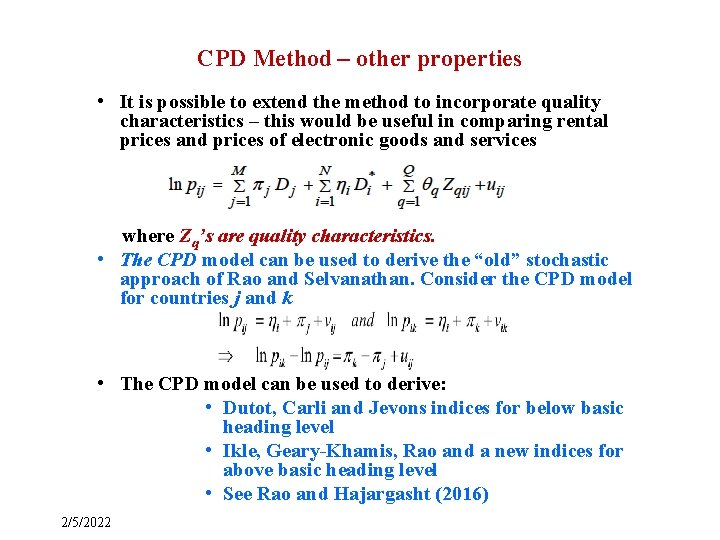
CPD Method – other properties • It is possible to extend the method to incorporate quality characteristics – this would be useful in comparing rental prices and prices of electronic goods and services where Zq’s are quality characteristics. • The CPD model can be used to derive the “old” stochastic approach of Rao and Selvanathan. Consider the CPD model for countries j and k • The CPD model can be used to derive: • Dutot, Carli and Jevons indices for below basic heading level • Ikle, Geary-Khamis, Rao and a new indices for above basic heading level • See Rao and Hajargasht (2016) 2/5/2022

Notation M countries and N commodities observed price of the i-th commodity in the j-th country quantity of the i-th commodity in the j-th country purchasing power parity of j-th country Average price for i-th commodity Expenditure shares Weights based on expenditure shares When M = 2, we have the case of binary comparisons.

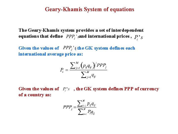
Geary-Khamis System of equations The Geary-Khamis system provides a set of interdependent equations that define and international prices , Given the values of , the GK system defines each international average price as: Given the values of of a country as: , the GK system defines PPP of currency

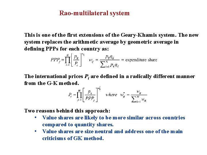
Rao-multilateral system This is one of the first extensions of the Geary-Khamis system. The new system replaces the arithmetic average by geometric average in defining PPPs for each country as: The international prices Pi are defined in a radically different manner from the G-K method. Two reasons behind this approach: • Value shares are likely to be more similar across countries compared to quantity shares. • Value shares are size neutral and address one of the main criticisms of GK method.

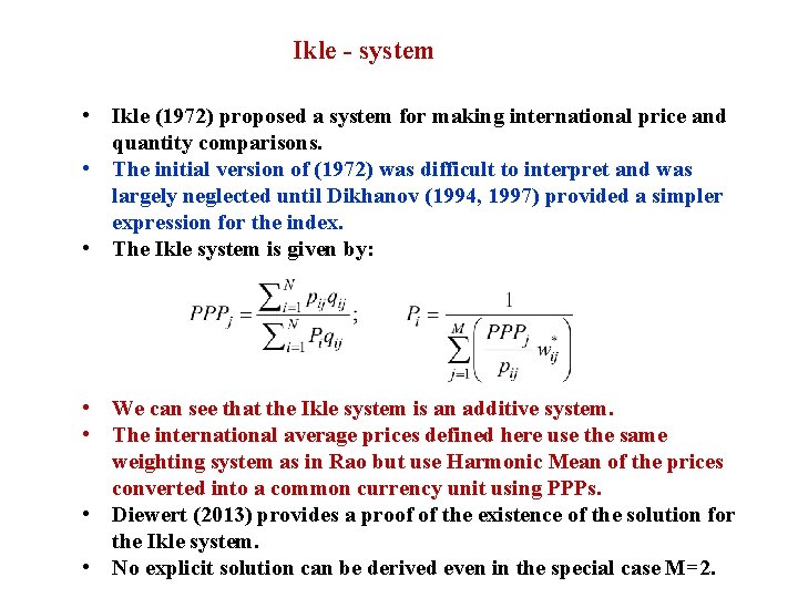
Ikle - system • Ikle (1972) proposed a system for making international price and quantity comparisons. • The initial version of (1972) was difficult to interpret and was largely neglected until Dikhanov (1994, 1997) provided a simpler expression for the index. • The Ikle system is given by: • We can see that the Ikle system is an additive system. • The international average prices defined here use the same weighting system as in Rao but use Harmonic Mean of the prices converted into a common currency unit using PPPs. • Diewert (2013) provides a proof of the existence of the solution for the Ikle system. • No explicit solution can be derived even in the special case M=2.

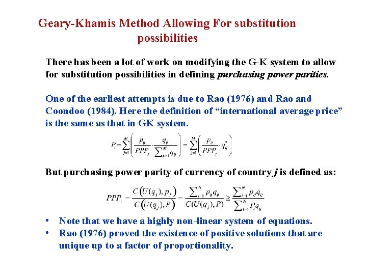
Geary-Khamis Method Allowing For substitution possibilities There has been a lot of work on modifying the G-K system to allow for substitution possibilities in defining purchasing power parities. One of the earliest attempts is due to Rao (1976) and Rao and Coondoo (1984). Here the definition of “international average price” is the same as that in GK system. But purchasing power parity of currency of country j is defined as: • Note that we have a highly non-linear system of equations. • Rao (1976) proved the existence of positive solutions that are unique up to a factor of proportionality.

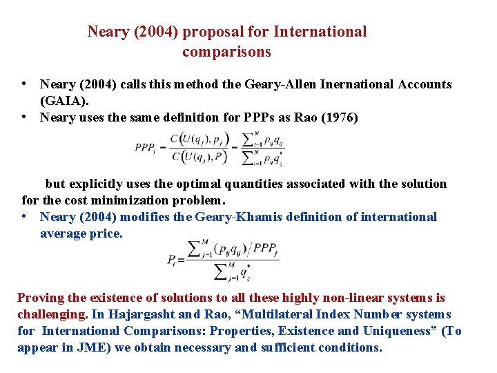
Neary (2004) proposal for International comparisons • Neary (2004) calls this method the Geary-Allen Inernational Accounts (GAIA). • Neary uses the same definition for PPPs as Rao (1976) but explicitly uses the optimal quantities associated with the solution for the cost minimization problem. • Neary (2004) modifies the Geary-Khamis definition of international average price. Proving the existence of solutions to all these highly non-linear systems is challenging. In Hajargasht and Rao, “Multilateral Index Number systems for International Comparisons: Properties, Existence and Uniqueness” (To appear in JME) we obtain necessary and sufficient conditions.

Reliability of PPPs from the International Comparison Program

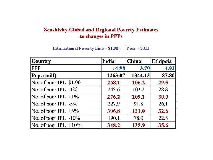
Sensitivity Global and Regional Poverty Estimates to changes in PPPs International Poverty Line = $1. 90; Year = 2011