Aggregate expenditure 1 Autonomous versus induced expenditure 2

Aggregate expenditure 1. Autonomous versus induced expenditure 2. The consumption function 3. The theory of investment 4. Government purchase function 5. The net export function

Autonomous versus induced Expenditure • Autonomous expenditure: The components of aggregate expenditure that do not change when real GDP changes. • Induced expenditure: The components of aggregate expenditure that change when real GDP changes.

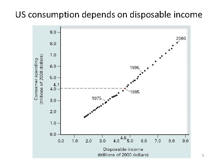
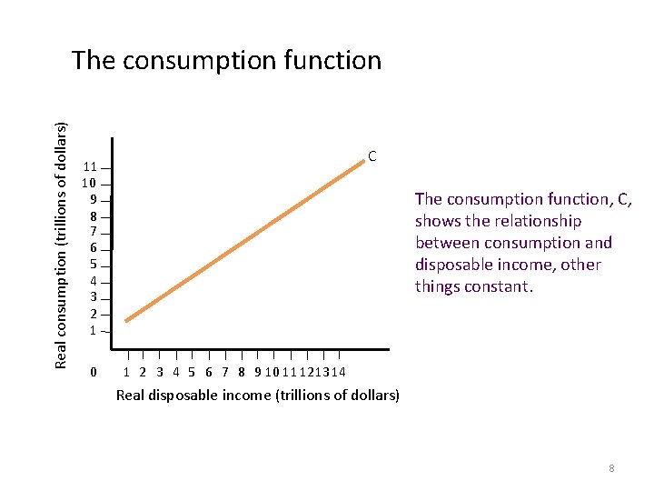
The consumption function reveals the relationship between consumption and disposable income, other things constant.

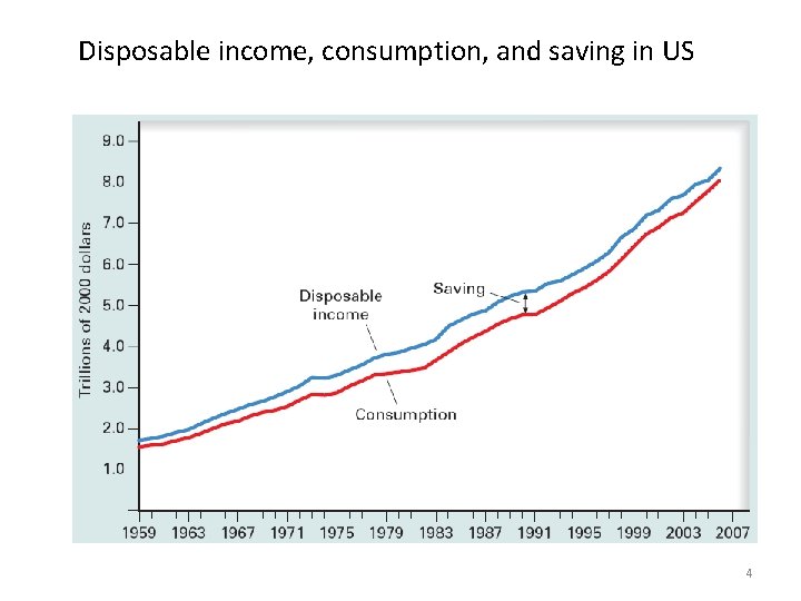
Disposable income, consumption, and saving in US 4

US consumption depends on disposable income 5

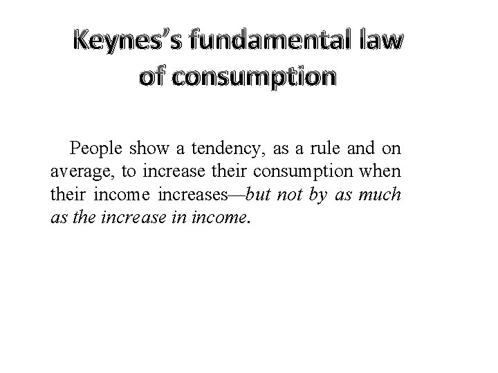
Keynes’s fundamental law of consumption People show a tendency, as a rule and on average, to increase their consumption when their income increases—but not by as much as the increase in income.

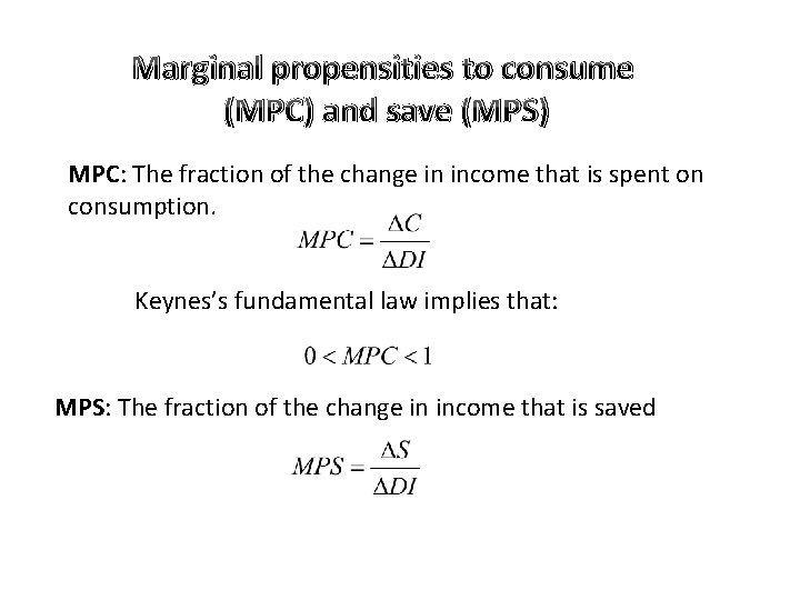
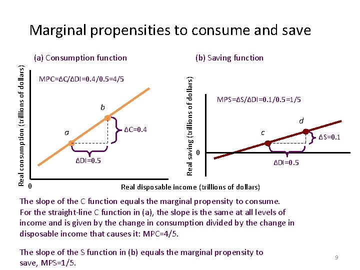
Marginal propensities to consume (MPC) and save (MPS) MPC: The fraction of the change in income that is spent on consumption. Keynes’s fundamental law implies that: MPS: The fraction of the change in income that is saved

Real consumption (trillions of dollars) The consumption function C 11 10 9 8 7 6 5 4 3 2 1 0 The consumption function, C, shows the relationship between consumption and disposable income, other things constant. 1 2 3 4 5 6 7 8 9 10 11 12 13 14 Real disposable income (trillions of dollars) 8

Marginal propensities to consume and save MPC=∆C/∆DI=0. 4/0. 5=4/5 b ∆C=0. 4 a ∆DI=0. 5 0 (b) Saving function Real saving (trillions of dollars) Real consumption (trillions of dollars) (a) Consumption function MPS=∆S/∆DI=0. 1/0. 5=1/5 d c ∆S=0. 1 0 ∆DI=0. 5 Real disposable income (trillions of dollars) The slope of the C function equals the marginal propensity to consume. For the straight-line C function in (a), the slope is the same at all levels of income and is given by the change in consumption divided by the change in disposable income that causes it: MPC=4/5. The slope of the S function in (b) equals the marginal propensity to save, MPS=1/5. 9

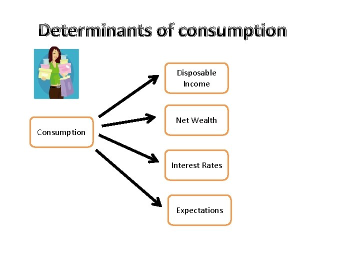
Determinants of consumption Disposable Income Net Wealth Consumption Interest Rates Expectations

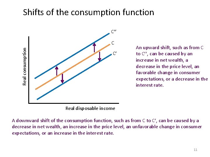
Shifts of the consumption function C’’ Real consumption C C’ An upward shift, such as from C to C’’, can be caused by an increase in net wealth, a decrease in the price level, an favorable change in consumer expectations, or a decrease in the interest rate. Real disposable income A downward shift of the consumption function, such as from C to C’, can be caused by a decrease in net wealth, an increase in the price level, an unfavorable change in consumer expectations, or an increase in the interest rate. 11

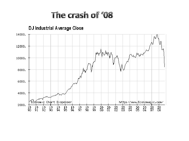
The crash of ‘ 08

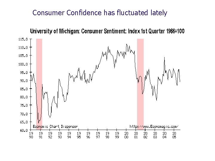
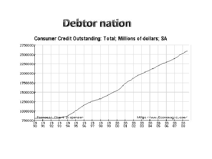
Let’s take out a loan so we can “cash out” some home equity. Rising home values have stimulated household borrowing and consumption in the past decade.

Consumer Confidence has fluctuated lately

Debtor nation

Theory of Investment Why do firms purchase things like new offshore drilling platforms, food processing plants, or bulldozers? Because they expect they can make a profit by doing so.

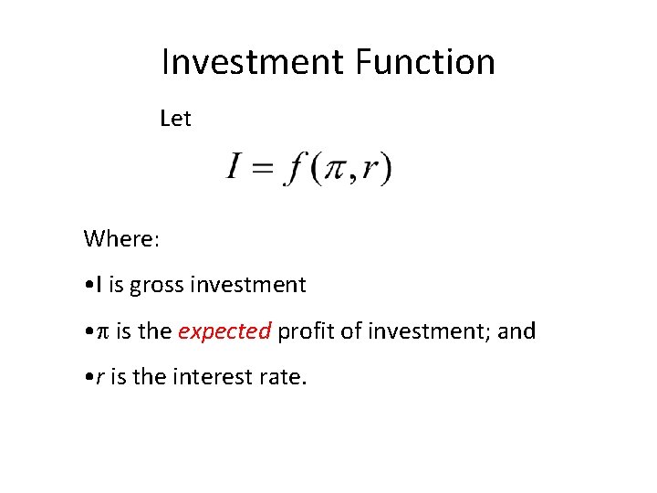
Investment Function Let Where: • I is gross investment • is the expected profit of investment; and • r is the interest rate.

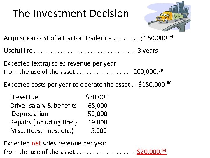
The Investment Decision Acquisition cost of a tractor–trailer rig. . . . $150, 000. 00 Useful life. . . . 3 years Expected (extra) sales revenue per year from the use of the asset. . . . 200, 000. 00 Expected costs per year to operate the asset. . $180, 000. 00 Diesel fuel Driver salary & benefits Depreciation Repairs (including tires) Misc. (fees, fines, etc. ) $38, 000 68, 000 50, 000 19, 000 5, 000 Expected net sales revenue per year from the use of the asset. . . . $20, 000. 00

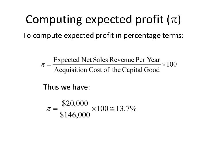
Computing expected profit ( ) To compute expected profit in percentage terms: Thus we have:

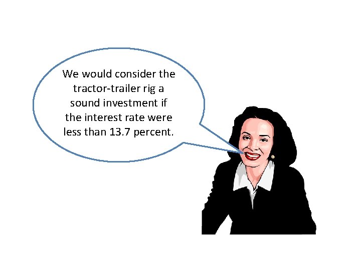
We would consider the tractor-trailer rig a sound investment if the interest rate were less than 13. 7 percent.

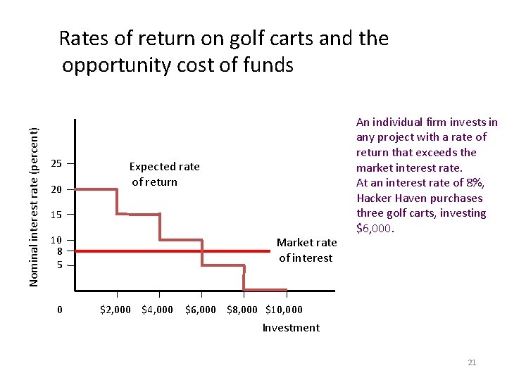
Nominal interest rate (percent) Rates of return on golf carts and the opportunity cost of funds 25 20 Expected rate of return 15 10 8 5 0 Market rate of interest $2, 000 $4, 000 An individual firm invests in any project with a rate of return that exceeds the market interest rate. At an interest rate of 8%, Hacker Haven purchases three golf carts, investing $6, 000 $8, 000 $10, 000 Investment 21

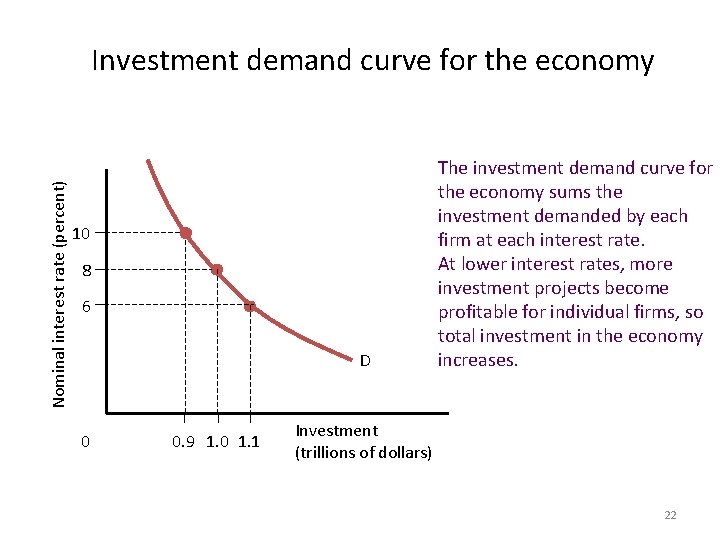
Nominal interest rate (percent) Investment demand curve for the economy 10 8 6 D 0 0. 9 1. 0 1. 1 The investment demand curve for the economy sums the investment demanded by each firm at each interest rate. At lower interest rates, more investment projects become profitable for individual firms, so total investment in the economy increases. Investment (trillions of dollars) 22

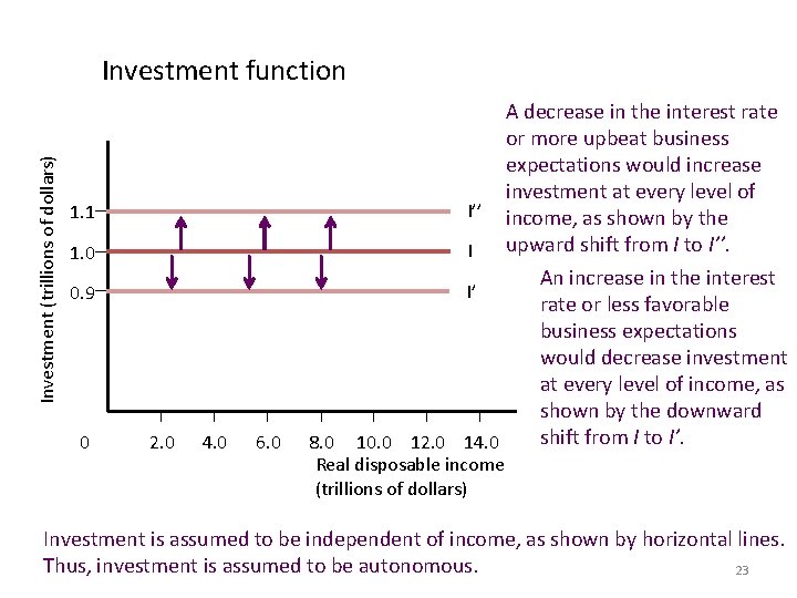
Investment (trillions of dollars) Investment function 1. 1 I’’ 1. 0 I 0. 9 I’ 0 2. 0 4. 0 6. 0 8. 0 10. 0 12. 0 14. 0 Real disposable income (trillions of dollars) A decrease in the interest rate or more upbeat business expectations would increase investment at every level of income, as shown by the upward shift from I to I’’. An increase in the interest rate or less favorable business expectations would decrease investment at every level of income, as shown by the downward shift from I to I’. Investment is assumed to be independent of income, as shown by horizontal lines. Thus, investment is assumed to be autonomous. 23

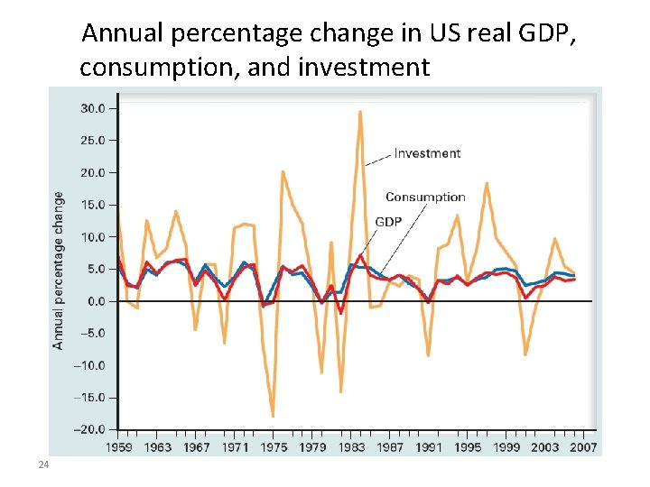
Annual percentage change in US real GDP, consumption, and investment 24

Government purchase function Because government purchases are controlled by public officials, we treat them as autonomous—that is, determined independent of income

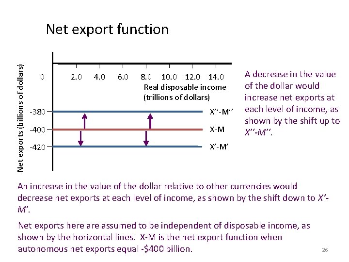
Net exports (billions of dollars) Net export function 0 2. 0 4. 0 6. 0 8. 0 10. 0 12. 0 14. 0 Real disposable income (trillions of dollars) -380 X’’-M’’ -400 X-M -420 X’-M’ A decrease in the value of the dollar would increase net exports at each level of income, as shown by the shift up to X’’-M’’. An increase in the value of the dollar relative to other currencies would decrease net exports at each level of income, as shown by the shift down to X’M’. Net exports here assumed to be independent of disposable income, as shown by the horizontal lines. X-M is the net export function when autonomous net exports equal -$400 billion. 26

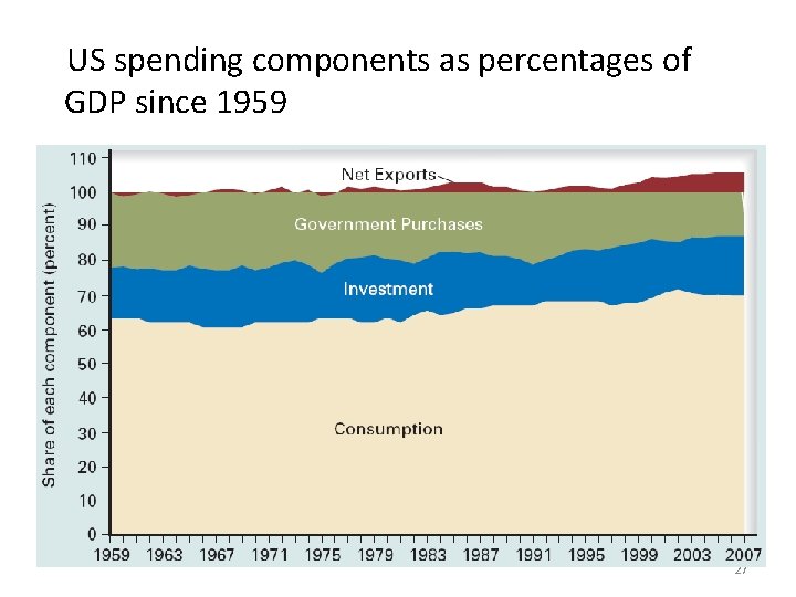
US spending components as percentages of GDP since 1959 27