Topic 9 Price Levels and the Exchange Rate

Topic 9 Price Levels and the Exchange Rate in the Long Run Slides prepared by Thomas Bishop Copyright © 2009 Pearson Addison-Wesley. All rights reserved.

Preview • Law of one price • Purchasing power parity • Long run model of exchange rates: monetary approach • Relationship between interest rates and inflation: Fisher effect • Shortcomings of purchasing power parity • Long run model of exchange rates: real exchange rate approach • Real interest rates Copyright © 2009 Pearson Addison-Wesley. All rights reserved. 2

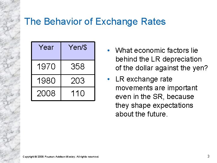
The Behavior of Exchange Rates Year Yen/$ 1970 358 1980 2008 203 110 Copyright © 2009 Pearson Addison-Wesley. All rights reserved. • What economic factors lie behind the LR depreciation of the dollar against the yen? • LR exchange rate movements are important even in the SR, because they shape expectations about the future. 3

The Behavior of Exchange Rates (cont. ) • We have seen that exchange rates are determined by interest rates and expectations about the future – which are influenced by national money markets. • To understand LR exchange rate movements, we must extend our model in two ways: (1) examine the linkages among monetary policy, inflation, interest rates, and exchange rates; and (2) examine how changes in the supply or demand for a country’s output will impact its currency. Copyright © 2009 Pearson Addison-Wesley. All rights reserved. 4

Law of One Price • The law of one price says that the same good in different competitive markets must sell for the same price, when transportation costs and barriers between those markets are not important. • Why? Suppose the price of pizza at one restaurant is $20, while the price of the same pizza at an identical restaurant across the street is $40. Ø What do you predict will happen? Ø Many people would buy the $20 pizza, few would buy the $40 one. Copyright © 2009 Pearson Addison-Wesley. All rights reserved. 5

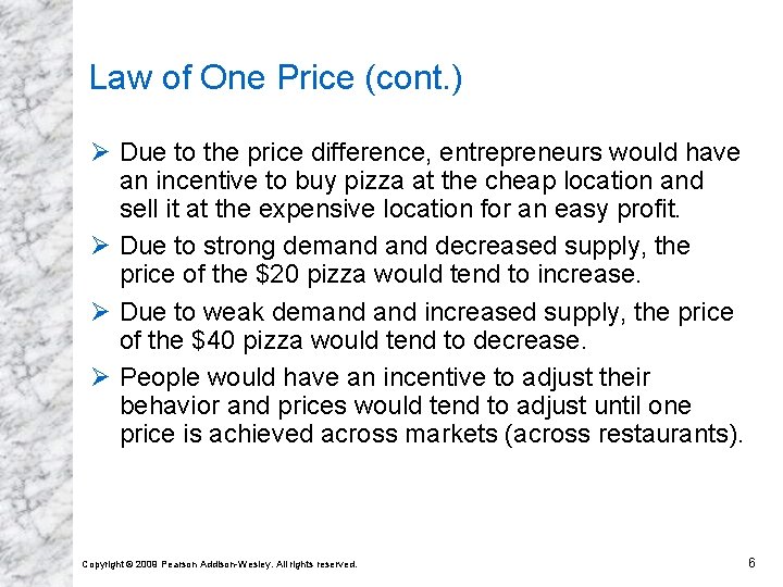
Law of One Price (cont. ) Ø Due to the price difference, entrepreneurs would have an incentive to buy pizza at the cheap location and sell it at the expensive location for an easy profit. Ø Due to strong demand decreased supply, the price of the $20 pizza would tend to increase. Ø Due to weak demand increased supply, the price of the $40 pizza would tend to decrease. Ø People would have an incentive to adjust their behavior and prices would tend to adjust until one price is achieved across markets (across restaurants). Copyright © 2009 Pearson Addison-Wesley. All rights reserved. 6

Law of One Price (cont. ) • Consider a pizza restaurant in Seattle and one across the border in Vancouver. • The law of one price says that the price of the same pizza (using a common currency to measure the price) in the two cities must be the same if markets are competitive and transportation costs and barriers between markets are not important. Ppizza. US = (EUS$/C$) x (Ppizza. Canada) Ppizza. US = price of pizza in Seattle Ppizza. Canada = price of pizza in Vancouver EUS$/C$ = US dollar/Canadian dollar exchange rate Copyright © 2009 Pearson Addison-Wesley. All rights reserved. 7

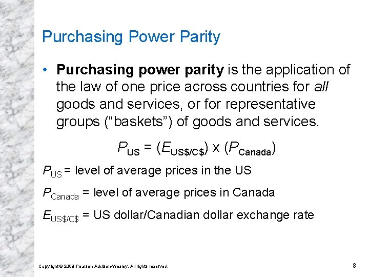
Purchasing Power Parity • Purchasing power parity is the application of the law of one price across countries for all goods and services, or for representative groups (“baskets”) of goods and services. PUS = (EUS$/C$) x (PCanada) PUS = level of average prices in the US PCanada = level of average prices in Canada EUS$/C$ = US dollar/Canadian dollar exchange rate Copyright © 2009 Pearson Addison-Wesley. All rights reserved. 8

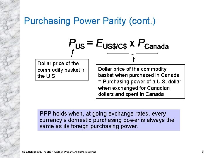
Purchasing Power Parity (cont. ) Dollar price of the commodity basket in the U. S. Dollar price of the commodity basket when purchased in Canada = Purchasing power of a U. S. dollar when exchanged for Canadian dollars and spent in Canada PPP holds when, at going exchange rates, every currency’s domestic purchasing power is always the same as its foreign purchasing power. Copyright © 2009 Pearson Addison-Wesley. All rights reserved. 9

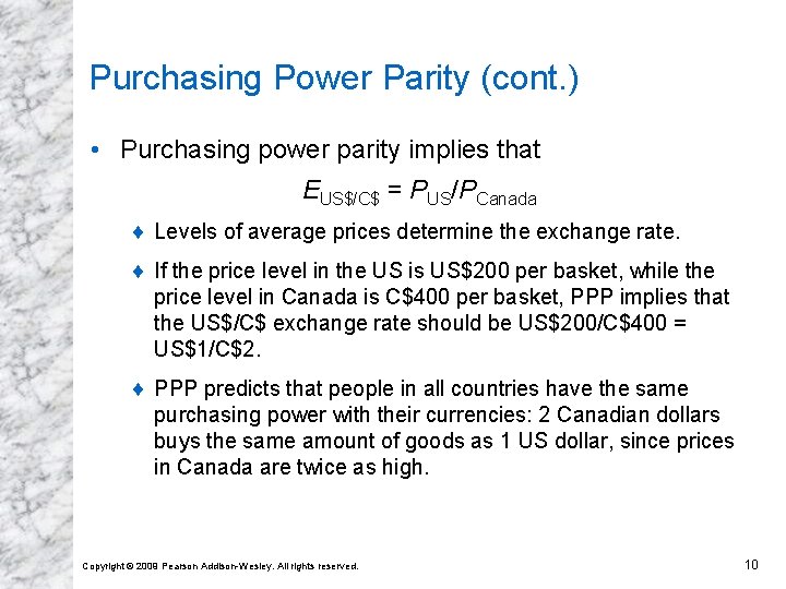
Purchasing Power Parity (cont. ) • Purchasing power parity implies that EUS$/C$ = PUS/PCanada ¨ Levels of average prices determine the exchange rate. ¨ If the price level in the US is US$200 per basket, while the price level in Canada is C$400 per basket, PPP implies that the US$/C$ exchange rate should be US$200/C$400 = US$1/C$2. ¨ PPP predicts that people in all countries have the same purchasing power with their currencies: 2 Canadian dollars buys the same amount of goods as 1 US dollar, since prices in Canada are twice as high. Copyright © 2009 Pearson Addison-Wesley. All rights reserved. 10

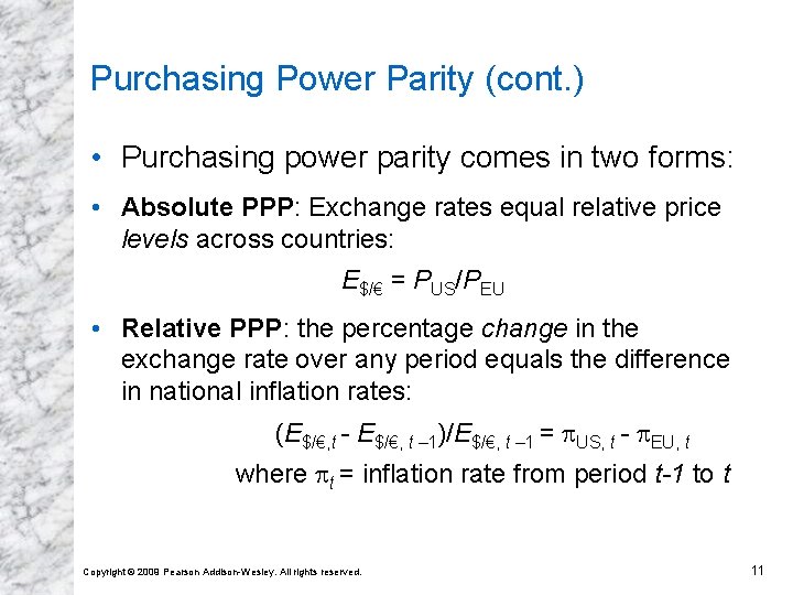
Purchasing Power Parity (cont. ) • Purchasing power parity comes in two forms: • Absolute PPP: Exchange rates equal relative price levels across countries: E$/€ = PUS/PEU • Relative PPP: the percentage change in the exchange rate over any period equals the difference in national inflation rates: (E$/€, t - E$/€, t – 1)/E$/€, t – 1 = US, t - EU, t where t = inflation rate from period t-1 to t Copyright © 2009 Pearson Addison-Wesley. All rights reserved. 11

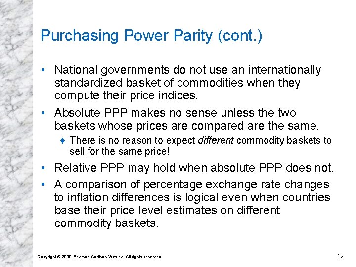
Purchasing Power Parity (cont. ) • National governments do not use an internationally standardized basket of commodities when they compute their price indices. • Absolute PPP makes no sense unless the two baskets whose prices are compared are the same. ¨ There is no reason to expect different commodity baskets to sell for the same price! • Relative PPP may hold when absolute PPP does not. • A comparison of percentage exchange rate changes to inflation differences is logical even when countries base their price level estimates on different commodity baskets. Copyright © 2009 Pearson Addison-Wesley. All rights reserved. 12

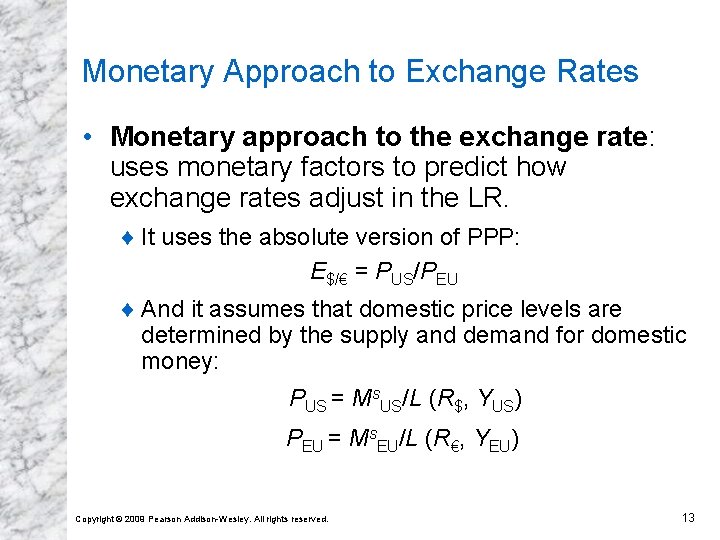
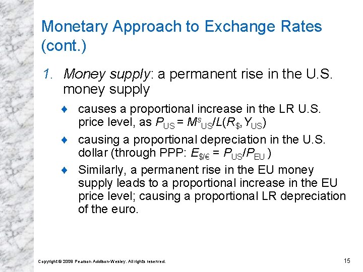
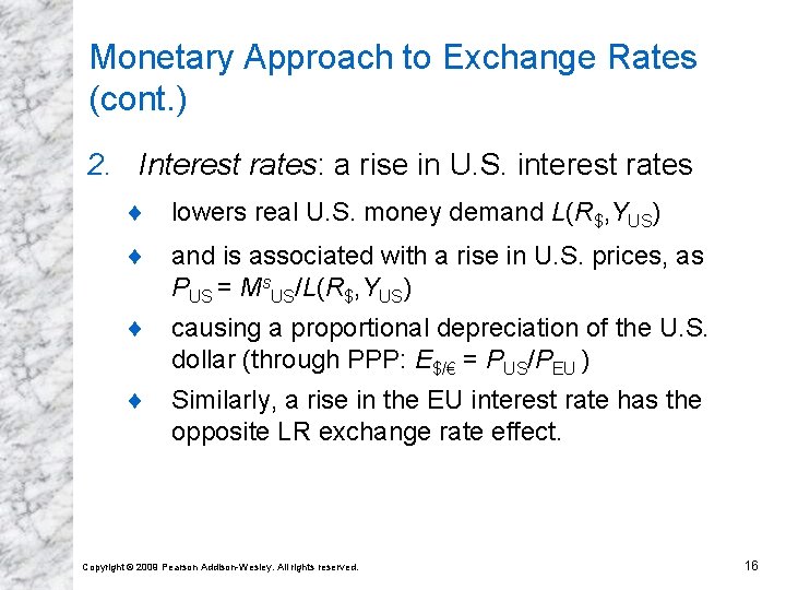
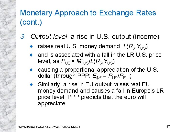
Monetary Approach to Exchange Rates • Monetary approach to the exchange rate: uses monetary factors to predict how exchange rates adjust in the LR. ¨ It uses the absolute version of PPP: E$/€ = PUS/PEU ¨ And it assumes that domestic price levels are determined by the supply and demand for domestic money: PUS = Ms. US/L (R$, YUS) PEU = Ms. EU/L (R€, YEU) Copyright © 2009 Pearson Addison-Wesley. All rights reserved. 13

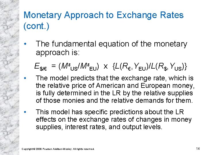
Monetary Approach to Exchange Rates (cont. ) • The fundamental equation of the monetary approach is: E$/€ = (Ms. US/Ms. EU) x {L(R€, YEU)/L(R$, YUS)} • The model predicts that the exchange rate, which is the relative price of American and European money, is fully determined in the LR by the relative supplies of those monies and the relative demands for them. • This model has specific predictions about the LR effects on the exchange rates of changes in money supplies, interest rates, and output levels. Copyright © 2009 Pearson Addison-Wesley. All rights reserved. 14

Monetary Approach to Exchange Rates (cont. ) 1. Money supply: a permanent rise in the U. S. money supply ¨ causes a proportional increase in the LR U. S. price level, as PUS = Ms. US/L(R$, YUS) ¨ causing a proportional depreciation in the U. S. dollar (through PPP: E$/€ = PUS/PEU ) ¨ Similarly, a permanent rise in the EU money supply leads to a proportional increase in the EU price level; causing a proportional LR depreciation of the euro. Copyright © 2009 Pearson Addison-Wesley. All rights reserved. 15

Monetary Approach to Exchange Rates (cont. ) 2. Interest rates: a rise in U. S. interest rates ¨ lowers real U. S. money demand L(R$, YUS) ¨ and is associated with a rise in U. S. prices, as PUS = Ms. US/L(R$, YUS) ¨ causing a proportional depreciation of the U. S. dollar (through PPP: E$/€ = PUS/PEU ) ¨ Similarly, a rise in the EU interest rate has the opposite LR exchange rate effect. Copyright © 2009 Pearson Addison-Wesley. All rights reserved. 16

Monetary Approach to Exchange Rates (cont. ) 3. Output level: a rise in U. S. output (income) ¨ raises real U. S. money demand, L(R$, YUS) ¨ and is associated with a fall in the LR U. S. price level, as PUS = Ms. US/L(R$, YUS) ¨ causing a proportional appreciation of the U. S. dollar (through PPP: E$/€ = PUS/PEU ) ¨ Similarly, a rise in EU output raises real EU money demand causes a fall in Europe’s LR price level. PPP predicts that the euro will appreciate. Copyright © 2009 Pearson Addison-Wesley. All rights reserved. 17

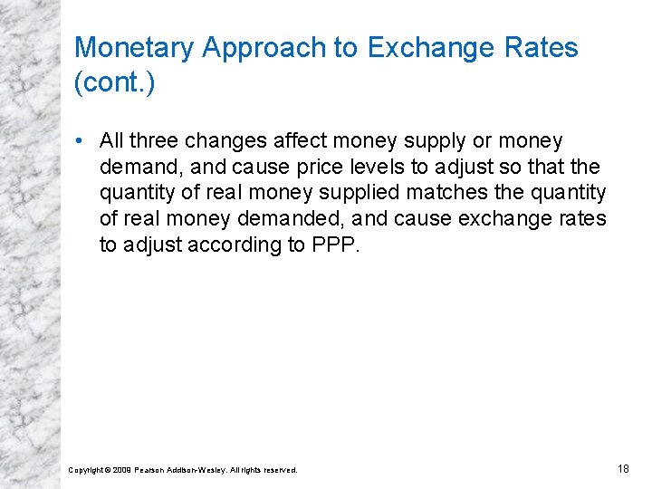
Monetary Approach to Exchange Rates (cont. ) • All three changes affect money supply or money demand, and cause price levels to adjust so that the quantity of real money supplied matches the quantity of real money demanded, and cause exchange rates to adjust according to PPP. Copyright © 2009 Pearson Addison-Wesley. All rights reserved. 18

Monetary Approach to Exchange Rates (cont. ) • A change in the level of the money supply results in a change in the price level. • A change in the growth rate of the money supply results in a change in the growth rate of prices (inflation). ¨ A constant growth rate in the money supply results in a persistent growth rate in prices (persistent inflation) at the same constant rate. ¨ Inflation does not affect the productive capacity of the economy in the LR. ¨ Inflation, however, does affect nominal interest rates. How? Copyright © 2009 Pearson Addison-Wesley. All rights reserved. 19

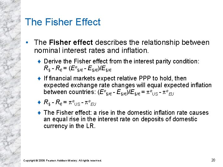
The Fisher Effect • The Fisher effect describes the relationship between nominal interest rates and inflation. ¨ Derive the Fisher effect from the interest parity condition: R$ - R€ = (Ee$/€ - E$/€)/E$/€ ¨ If financial markets expect relative PPP to hold, then expected exchange rate changes will equal expected inflation between countries: (Ee$/€ - E$/€)/E$/€ = e. US - e. EU ¨ R$ - R€ = e. US - e. EU ¨ The Fisher effect: a rise in the domestic inflation rate causes an equal rise in the interest rate on deposits of domestic currency in the LR. Copyright © 2009 Pearson Addison-Wesley. All rights reserved. 20

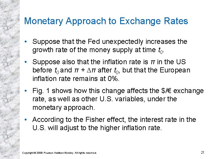
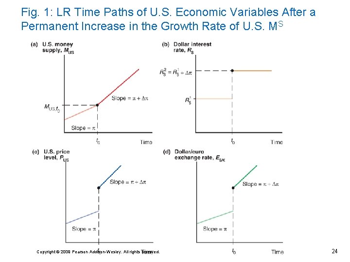
Monetary Approach to Exchange Rates • Suppose that the Fed unexpectedly increases the growth rate of the money supply at time t 0. • Suppose also that the inflation rate is π in the US before t 0 and π + π after t 0, but that the European inflation rate remains at 0%. • Fig. 1 shows how this change affects the $/€ exchange rate, as well as other U. S. variables, under the monetary approach. • According to the Fisher effect, the interest rate in the U. S. will adjust to the higher inflation rate. Copyright © 2009 Pearson Addison-Wesley. All rights reserved. 21

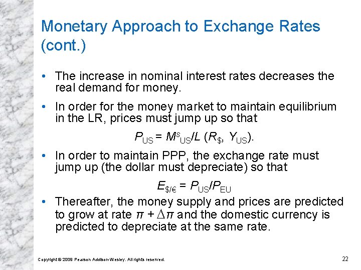
Monetary Approach to Exchange Rates (cont. ) • The increase in nominal interest rates decreases the real demand for money. • In order for the money market to maintain equilibrium in the LR, prices must jump up so that PUS = Ms. US/L (R$, YUS). • In order to maintain PPP, the exchange rate must jump up (the dollar must depreciate) so that E$/€ = PUS/PEU • Thereafter, the money supply and prices are predicted to grow at rate π + π and the domestic currency is predicted to depreciate at the same rate. Copyright © 2009 Pearson Addison-Wesley. All rights reserved. 22

Monetary Approach to Exchange Rates (cont. ) • How does the foreign exchange market react at time t 0? • People now expect more rapid future money supply growth and dollar depreciation. • Investors respond by moving into foreign deposits, which momentarily offer higher expected returns. • This causes the dollar to depreciate in the foreign exchange market, moving to a new trend line along which depreciation is more rapid than it was up to time t 0. Copyright © 2009 Pearson Addison-Wesley. All rights reserved. 23

Fig. 1: LR Time Paths of U. S. Economic Variables After a Permanent Increase in the Growth Rate of U. S. MS Copyright © 2009 Pearson Addison-Wesley. All rights reserved. 24

The Role of Inflation and Expectations In the LR model without PPP: • A permanent increase in the U. S. money supply eventually leads to a rise in the U. S. price level. • No inflation is predicted to occur in the LR, but only during the transition to the LR equilibrium. • During the transition, inflation causes the nominal interest rate to increase to its LR value. • Expectations of higher U. S. inflation cause the expected return on euro deposits to increase, making the dollar depreciate before the transition period. Copyright © 2009 Pearson Addison-Wesley. All rights reserved. 25

The Role of Inflation and Expectations (cont. ) • In the monetary approach (with PPP), the rate of inflation increases permanently when the growth rate of the U. S. money supply increases permanently. • With persistent U. S. inflation (above European inflation), the monetary approach also predicts an increase in the U. S. nominal interest rate. • Expectations of higher U. S. inflation cause the expected purchasing power of the dollar to decrease relative to the expected purchasing power of the euro, thereby making the dollar depreciate. Copyright © 2009 Pearson Addison-Wesley. All rights reserved. 26

The Role of Inflation and Expectations (cont. ) • In the LR model without PPP, the U. S. price level does not immediately adjust even if expectations of inflation adjust, ¨ causing the exchange rate to overshoot (causing the dollar to depreciate more than) its LR value. • In the monetary approach (with PPP), the price level adjusts immediately with expectations of inflation, ¨ causing the domestic currency to depreciate, but with no overshooting. Copyright © 2009 Pearson Addison-Wesley. All rights reserved. 27

Shortcomings of PPP • There is scant empirical support for absolute PPP. ¨ The prices of identical commodity baskets, when converted to a single currency, differ substantially across countries. • Even the law of one price (which forms the basis for absolute PPP) performs poorly when looking at recent data. ¨ Since the 1970 s, very similar manufactured goods have sold for widely different prices in various countries. Copyright © 2009 Pearson Addison-Wesley. All rights reserved. 28

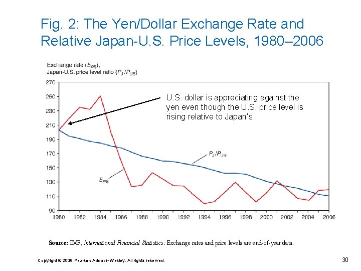
Shortcomings of PPP (cont. ) • Relative PPP is more consistent with the data, but it also performs poorly to predict exchange rates. • Fig. 2 shows the yen/dollar exchange rate and the ratio of Japanese and U. S. price levels from 1980 to 2006. • Relative PPP predicts that EY/$ and PJ /PUS should move in proportion, but clearly they do not. ¨ In the early 1980 s, there was a steep appreciation of the dollar even though Japan’s price level was consistently falling relative to that in the U. S. ¨ Relative PPP predicts that the $ should have depreciated! Copyright © 2009 Pearson Addison-Wesley. All rights reserved. 29

Fig. 2: The Yen/Dollar Exchange Rate and Relative Japan-U. S. Price Levels, 1980– 2006 U. S. dollar is appreciating against the yen even though the U. S. price level is rising relative to Japan’s. Source: IMF, International Financial Statistics. Exchange rates and price levels are end-of-year data. Copyright © 2009 Pearson Addison-Wesley. All rights reserved. 30

Shortcomings of PPP (cont. ) • Reasons why PPP may not be accurate: the law of one price may not hold because of: 1. Transport costs and trade restrictions 2. Imperfect competition 3. Inflation data reported in different countries are based on different commodity baskets Copyright © 2009 Pearson Addison-Wesley. All rights reserved. 31

Shortcomings of PPP (cont. ) 1. Trade barriers and non-tradable products • Transport costs and governmental trade restrictions make trade expensive and in some cases create non -tradable goods or services. • Nontradables are primarily services and housing which are generally offered within a limited geographic region (e. g. , haircuts, doctor’s visits, or rent). • The existence in all countries of nontradables whose prices are not linked internationally allows systematic deviations from PPP. • One price need not hold in two markets. Copyright © 2009 Pearson Addison-Wesley. All rights reserved. 32

Shortcomings of PPP (cont. ) 2. Imperfect competition may result in price discrimination by monopolistic or oligopolistic firms • A monopolist sells the same product for different prices in different markets to maximize profits. ¨ • Wealthy countries where demand is less price-elastic will be charged higher prices than poorer countries where demand is more price-elastic. One price need not hold in two markets. Copyright © 2009 Pearson Addison-Wesley. All rights reserved. 33

Shortcomings of PPP (cont. ) 3. Differences in consumption patterns and price level measurement • Government measures of the price level differ from country to country. ¨ • People living in different countries consume different goods and services, so the government reference commodity basket is different. One price need not hold in two markets. Copyright © 2009 Pearson Addison-Wesley. All rights reserved. 34

Case Study: Why Price Levels are Lower in Poorer Countries • Data consistently show that price levels (when expressed in terms of a single currency) are positively related to the level of real income per capita. ¨ A dollar when converted to a local currency at the market exchange rate, generally goes much farther in a poor country than in a rich one. • Data also show that nontradables tend to be more expensive (relative to tradables) in richer countries. • Why? Balassa-Samuelson theory: poor-country workers are less productive than rich-country workers in the tradables sector but have similar productivity in the nontradables sector. Copyright © 2009 Pearson Addison-Wesley. All rights reserved. 35

Case Study: Why Price Levels are Lower in Poorer Countries (cont. ) • Prices of traded goods are roughly equal in all countries. • However, the lower labor productivity in the tradables sector of poor countries implies they have lower wages than rich countries, and therefore lower production costs for nontradables; and a lower price of nontradables. • Rich countries with higher labor productivity in the tradables sector will tend to have higher nontradable prices and higher price levels. Copyright © 2009 Pearson Addison-Wesley. All rights reserved. 36

Case Study: Why Price Levels are Lower in Poorer Countries (cont. ) • Alternatively, Bhagwati-Kravis-Lipsey posit that rich countries have a higher K/L ratio than poor countries. • The MPL (and thereby wages) will be higher in rich countries. • Nontradables consist largely of services which are labor intensive. So nontradables will be cheaper in poor countries because they have more labor. • Both theories suggests that overall price levels (when measured by a single currency) will be higher in rich countries than in poor. Copyright © 2009 Pearson Addison-Wesley. All rights reserved. 37

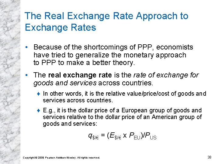
The Real Exchange Rate Approach to Exchange Rates • Because of the shortcomings of PPP, economists have tried to generalize the monetary approach to PPP to make a better theory. • The real exchange rate is the rate of exchange for goods and services across countries. ¨ In other words, it is the relative value/price/cost of goods and services across countries. ¨ E. g. , it is the dollar price of a European group of goods and services relative to the dollar price of an American group of goods and services: q$/€ = (E$/€ x PEU)/PUS Copyright © 2009 Pearson Addison-Wesley. All rights reserved. 38

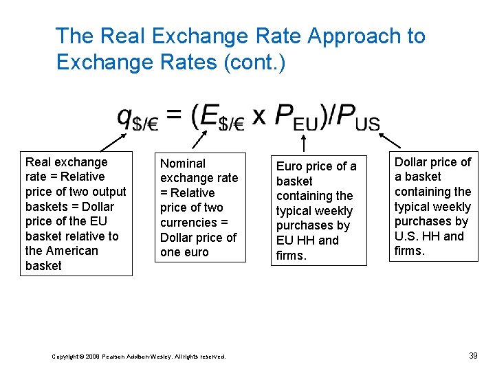
The Real Exchange Rate Approach to Exchange Rates (cont. ) Real exchange rate = Relative price of two output baskets = Dollar price of the EU basket relative to the American basket Nominal exchange rate = Relative price of two currencies = Dollar price of one euro Copyright © 2009 Pearson Addison-Wesley. All rights reserved. Euro price of a basket containing the typical weekly purchases by EU HH and firms. Dollar price of a basket containing the typical weekly purchases by U. S. HH and firms. 39

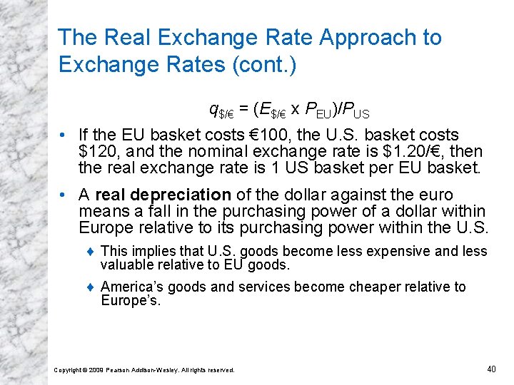
The Real Exchange Rate Approach to Exchange Rates (cont. ) q$/€ = (E$/€ x PEU)/PUS • If the EU basket costs € 100, the U. S. basket costs $120, and the nominal exchange rate is $1. 20/€, then the real exchange rate is 1 US basket per EU basket. • A real depreciation of the dollar against the euro means a fall in the purchasing power of a dollar within Europe relative to its purchasing power within the U. S. ¨ This implies that U. S. goods become less expensive and less valuable relative to EU goods. ¨ America’s goods and services become cheaper relative to Europe’s. Copyright © 2009 Pearson Addison-Wesley. All rights reserved. 40

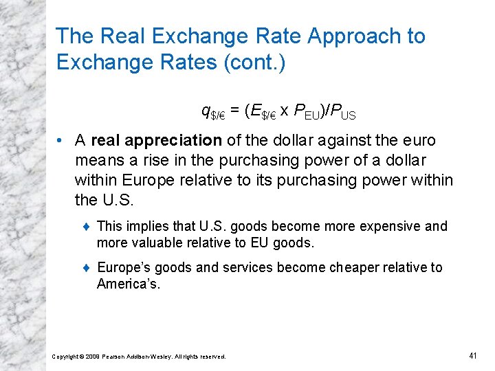
The Real Exchange Rate Approach to Exchange Rates (cont. ) q$/€ = (E$/€ x PEU)/PUS • A real appreciation of the dollar against the euro means a rise in the purchasing power of a dollar within Europe relative to its purchasing power within the U. S. ¨ This implies that U. S. goods become more expensive and more valuable relative to EU goods. ¨ Europe’s goods and services become cheaper relative to America’s. Copyright © 2009 Pearson Addison-Wesley. All rights reserved. 41

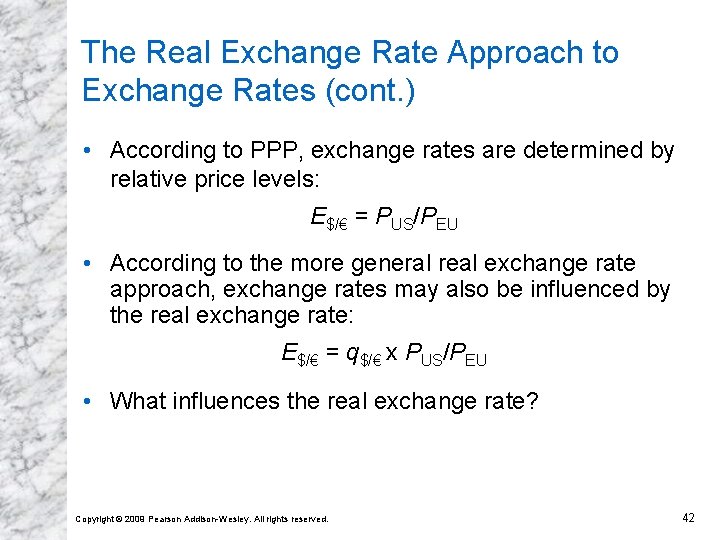
The Real Exchange Rate Approach to Exchange Rates (cont. ) • According to PPP, exchange rates are determined by relative price levels: E$/€ = PUS/PEU • According to the more general real exchange rate approach, exchange rates may also be influenced by the real exchange rate: E$/€ = q$/€ x PUS/PEU • What influences the real exchange rate? Copyright © 2009 Pearson Addison-Wesley. All rights reserved. 42

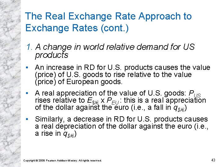
The Real Exchange Rate Approach to Exchange Rates (cont. ) 1. A change in world relative demand for US products • An increase in RD for U. S. products causes the value (price) of U. S. goods to rise relative to the value (price) of European goods. • A real appreciation of the value of U. S. goods: PUS rises relative to E$/€ x PEU : this is a real appreciation of the dollar against the euro (i. e. , a fall in q$/€) • Similarly, a decrease in RD for U. S. products causes a real depreciation of the dollar against the euro (i. e. , a rise in q$/€) Copyright © 2009 Pearson Addison-Wesley. All rights reserved. 43

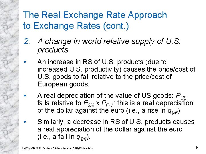
The Real Exchange Rate Approach to Exchange Rates (cont. ) 2. A change in world relative supply of U. S. products • An increase in RS of U. S. products (due to increased U. S. productivity) causes the price/cost of U. S. goods to fall relative to the price/cost of European goods. • A real depreciation of the value of US goods: PUS falls relative to E$/€ x PEU : this is a real depreciation of the dollar against the euro (i. e. , a rise in q$/€) • Similarly, a decrease in RS of U. S. products causes a real appreciation of the dollar against the euro (i. e. , a fall in q$/€). Copyright © 2009 Pearson Addison-Wesley. All rights reserved. 44

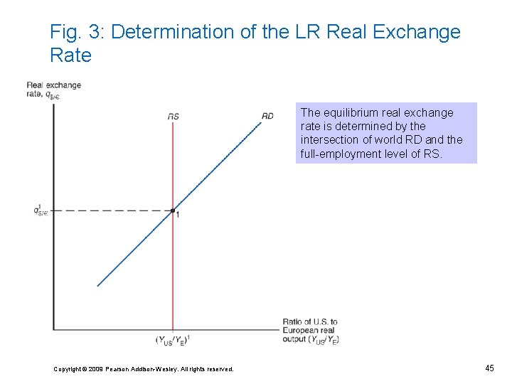
Fig. 3: Determination of the LR Real Exchange Rate The equilibrium real exchange rate is determined by the intersection of world RD and the full-employment level of RS. Copyright © 2009 Pearson Addison-Wesley. All rights reserved. 45

The Real Exchange Rate Approach to Exchange Rates (cont. ) • The RS curve in Fig. 3 is vertical because it is not impacted by the real exchange rate. ¨ The LR supply of goods and services in each country depends on factors of production like T, L, K, raw materials, and technology -not on prices or exchange rates. • The RD curve has a positive slope. ¨ American products become cheaper relative to European products as the real exchange rate rises. So a fall in the relative price of U. S. goods is associated with a rise in q$/€. Copyright © 2009 Pearson Addison-Wesley. All rights reserved. 46

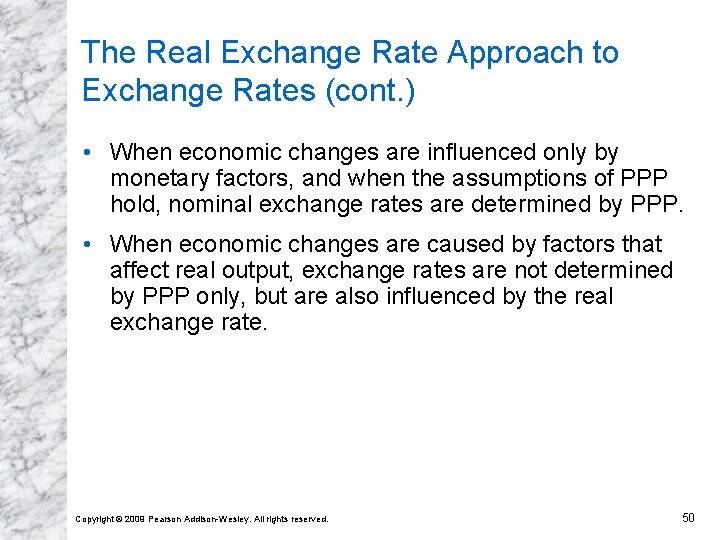
The Real Exchange Rate Approach to Exchange Rates (cont. ) • The real exchange rate is a more general approach to explain exchange rates. Both monetary factors and real (nonmonetary) factors influence nominal exchange rates. • The most important determinants of LR swings in nominal exchange rates are: 1. A shift in relative money supply levels. 2. A shift in relative money supply growth rates. 3. A change in relative output demand. 4. A change in relative output supply. Copyright © 2009 Pearson Addison-Wesley. All rights reserved. 47

The Real Exchange Rate Approach to Exchange Rates (cont. ) • What are the effects on the nominal exchange rate? E$/€ = q$/€ x PUS/PEU • When only monetary factors change and PPP holds, we have the same predictions as before (when using the monetary approach). ¨ no changes in the real exchange rate occurs • When factors influencing real output change, the real exchange rate changes. ¨ With an increase in RD for domestic products, the real exchange rate falls which causes nominal exchange rates to fall. ¨ With an increase in RS of domestic products, the situation is more complicated… Copyright © 2009 Pearson Addison-Wesley. All rights reserved. 48

The Real Exchange Rate Approach to Exchange Rates (cont. ) • With an increase in the RS of domestic products, the real exchange rate rises to make the price/cost of domestic goods depreciate, but also the relative amount of domestic output increases. ¨ This second effect increases the real demand for money in the domestic economy: PUS = Ms. US/L (R$, YUS) ¨ Thus, the domestic price level is predicted to decrease relative to the foreign price level. ¨ The effect on the nominal exchange rate is ambiguous: E$/€ = q$/€ x PUS/PEU ? Copyright © 2009 Pearson Addison-Wesley. All rights reserved. 49

The Real Exchange Rate Approach to Exchange Rates (cont. ) • When economic changes are influenced only by monetary factors, and when the assumptions of PPP hold, nominal exchange rates are determined by PPP. • When economic changes are caused by factors that affect real output, exchange rates are not determined by PPP only, but are also influenced by the real exchange rate. Copyright © 2009 Pearson Addison-Wesley. All rights reserved. 50

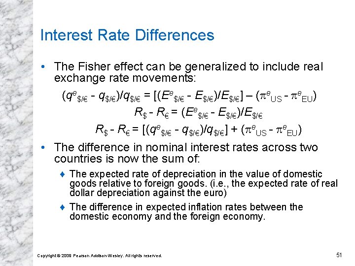
Interest Rate Differences • The Fisher effect can be generalized to include real exchange rate movements: (qe$/€ - q$/€)/q$/€ = [(Ee$/€ - E$/€)/E$/€] – ( e. US - e. EU) R$ - R€ = (Ee$/€ - E$/€)/E$/€ R$ - R€ = [(qe$/€ - q$/€)/q$/€] + ( e. US - e. EU) • The difference in nominal interest rates across two countries is now the sum of: ¨ The expected rate of depreciation in the value of domestic goods relative to foreign goods. (i. e. , the expected rate of real dollar depreciation against the euro) ¨ The difference in expected inflation rates between the domestic economy and the foreign economy. Copyright © 2009 Pearson Addison-Wesley. All rights reserved. 51

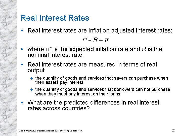
Real Interest Rates • Real interest rates are inflation-adjusted interest rates: re = R – π e • where πe is the expected inflation rate and R is the nominal interest rate. • Real interest rates are measured in terms of real output: ¨ the quantity of goods and services that savers can purchase when their assets pay interest ¨ the quantity of goods and services that borrowers can not purchase when they must pay interest on their loans • What are the predicted differences in real interest rates across countries? Copyright © 2009 Pearson Addison-Wesley. All rights reserved. 52

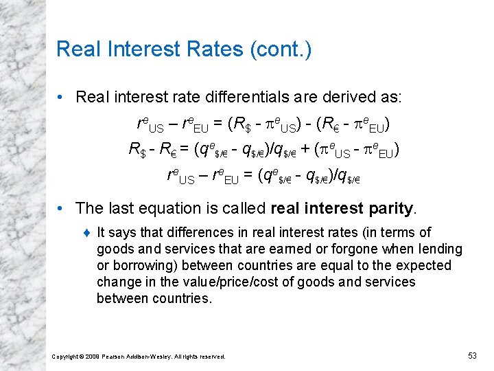
Real Interest Rates (cont. ) • Real interest rate differentials are derived as: re. US – re. EU = (R$ - e. US) - (R€ - e. EU) R$ - R€ = (qe$/€ - q$/€)/q$/€ + ( e. US - e. EU) re. US – re. EU = (qe$/€ - q$/€)/q$/€ • The last equation is called real interest parity. ¨ It says that differences in real interest rates (in terms of goods and services that are earned or forgone when lending or borrowing) between countries are equal to the expected change in the value/price/cost of goods and services between countries. Copyright © 2009 Pearson Addison-Wesley. All rights reserved. 53