On decisionmaking without regret routing games and convergence

On decision-making without regret, routing games, and convergence to equilibria Avrim Blum Carnegie Mellon University [Talk includes work joint with Eyal Even-Dar, Katrina Ligett, Yishay Mansour, and Brendan Mc. Mahan]

Online learning and game theory Avrim Blum Carnegie Mellon University [Talk includes work joint with Eyal Even-Dar, Katrina Ligett, Yishay Mansour, and Brendan Mc. Mahan]

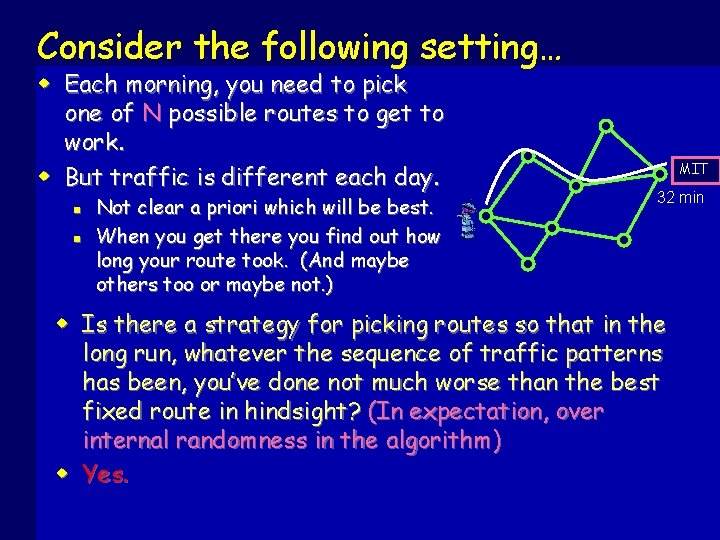
Consider the following setting… w Each morning, you need to pick one of N possible routes to get to work. w But traffic is different each day. n n Not clear a priori which will be best. When you get there you find out how long your route took. (And maybe others too or maybe not. ) MIT 32 min w Is there a strategy for picking routes so that in the long run, whatever the sequence of traffic patterns has been, you’ve done not much worse than the best fixed route in hindsight? (In expectation, over internal randomness in the algorithm) w Yes.

In fact, results of this sort have been known for a long time… Plan for this talk: 1. History and background on these “noregret” algorithms. 2. Some recent results / new directions. 3. Connections to game-theoretic equilibria (correlated equilibria, Nash equilibria in some cases) Talk is combination of classic and new work. Talk-version of survey chapter that Yishay Mansour and I are writing….

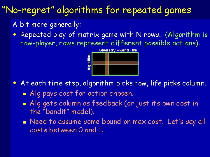
“No-regret” algorithms for repeated games A bit more generally: w Repeated play of matrix game with N rows. (Algorithm is row-player, rows represent different possible actions). Algorithm Adversary – world - life w At each time step, algorithm picks row, life picks column. n Alg pays cost for action chosen. n Alg gets column as feedback (or just its own cost in the “bandit” model). n Need to assume some bound on max cost. Let’s say all costs between 0 and 1.

“No-regret” algorithms for repeated games w At each time step, algorithm picks row, life picks column. Define average regret in T time steps as: n Alg pays cost for action chosen. (avg per-day cost of alg) – (avg per-day cost of best n Alg gets column as feedback (or just its own cost in fixed row in hindsight). the “bandit” model). We want this to go to 0 or better as T gets large [= “non Need to assume some bound on max cost. Let’s say all regret” algorithm]. costs between 0 and 1.

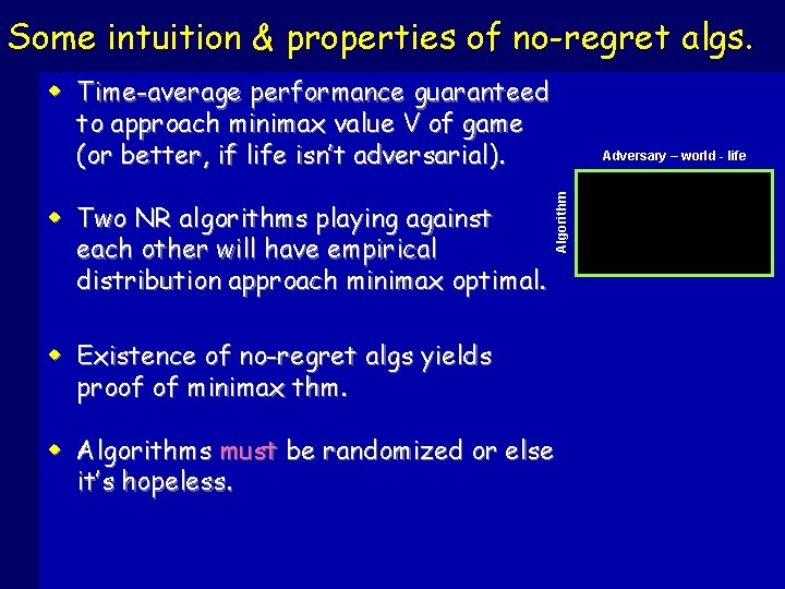
Some intuition & properties of no-regret algs. w Time-average performance guaranteed to approach minimax value V of game (or better, if life isn’t adversarial). Algorithm w Two NR algorithms playing against each other will have empirical distribution approach minimax optimal. Adversary – world - life w Existence of no-regret algs yields proof of minimax thm. w Algorithms must be randomized or else it’s hopeless.

History and development (abridged) w [Hannan’ 57, Blackwell’ 56]: Alg. with regret O((N/T)1/2). 2 n Re-phrasing, need only T = O(N/ ) steps to get timeaverage regret down to . (will call this quantity T ) n Optimal dependence on T (or ). Game-theorists viewed #rows N as constant, not so important as T, so pretty much done. w Learning-theory 80 s-90 s: “combining expert advice” n Perform (nearly) as well as best f 2 C. View N as large. n [Littlestone. Warmuth’ 89]: Weighted-majority algorithm l E[cost] · OPT(1+ ) + (log N)/ · OPT+ T+(log N)/ l Regret O((log N)/T)1/2. T = O((log N)/ 2). n Optimal as fn of N too, plus lots of work on exact constants, 2 nd order terms, etc. [CFHHSW 93]… w Extensions to bandit model (adds extra factor of N).

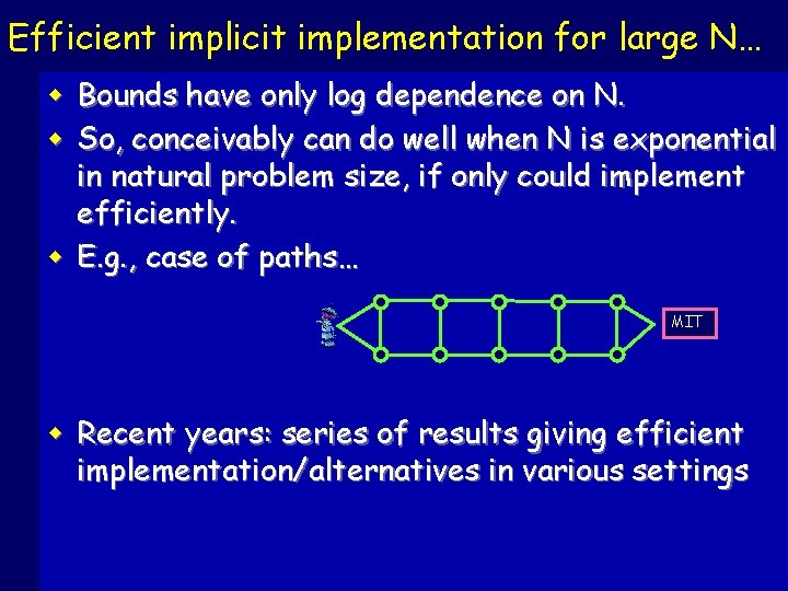
Efficient implicit implementation for large N… w Bounds have only log dependence on N. w So, conceivably can do well when N is exponential in natural problem size, if only could implement efficiently. w E. g. , case of paths… MIT w Recent years: series of results giving efficient implementation/alternatives in various settings

Efficient implicit implementation for large N… [Helmbold. Schapire 97]: best pruning of given DT. n [BChawla. Kalai 02]: 1+ static-optimal for list-update n [Takimoto. Warmuth 02]: online shortest path in DAGs. n [Kalai. Vempala 03]: elegant setting generalizing all above l Onlinear programming, more general online optimization (offline ) online) n [Zinkevich 03]: online convex programming w Recent years: series ofc. Mahan results giving efficient n [Awerbuch Kleinberg 04][M B 04]: [KV]!bandit model implementation/alternatives various settings: n [Kleinberg, Flaxman. Kalai. Mc. Mahan 05]: in [Z 03] ! bandit model n [Dani. Hayes 06]: faster convergence for [MB] n

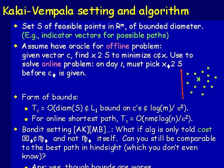
Kalai-Vempala setting and algorithm w Set S of feasible points in Rm, of bounded diameter. (E. g. , indicator vectors for possible paths) w Assume have oracle for offline problem: given vector c, find x 2 S to minimize c¢x. Use to solve online problem: on day t, must pick xt 2 S before ct is given. x w Form of bounds: 2 n T = O(diam(S) ¢ L 1 bound on c’s ¢ log(m)/ ). 2 n For online shortest path, T = O(nm¢log(n)/ ). w Bandit setting [AK][MB]…: What if alg is only told cost xt¢ct and not ct itself. Can you still be comparable to the best path in hindsight (which you don’t even know)?

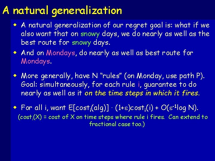
A natural generalization w A natural generalization of our regret goal is: what if we also want that on snowy days, we do nearly as well as the best route for snowy days. w And on Mondays, do nearly as well as best route for Mondays. w More generally, have N “rules” (on Monday, use path P). Goal: simultaneously, for each rule i, guarantee to do nearly as well as it on the time steps in which it fires. w For all i, want E[costi(alg)] · (1+ )costi(i) + O( -1 log N). (costi(X) = cost of X on time steps where rule i fires. Can extend to fractional case too. )

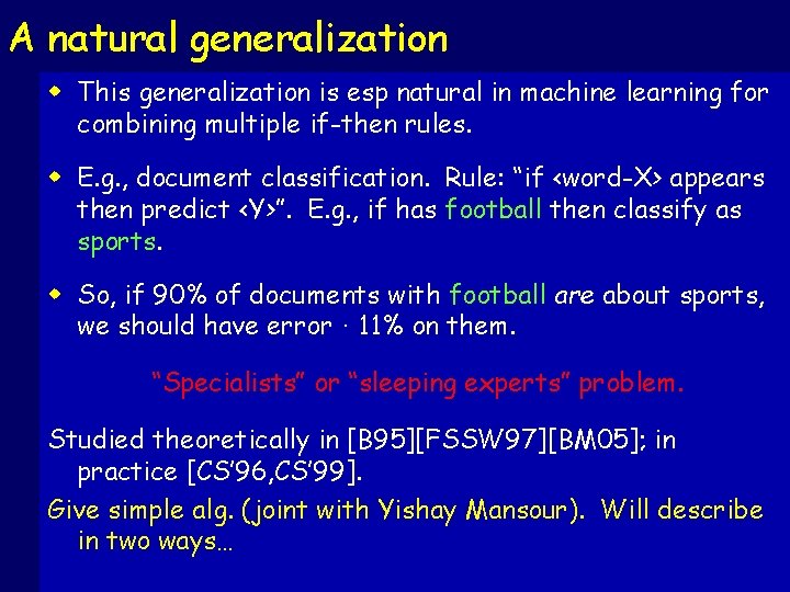
A natural generalization w This generalization is esp natural in machine learning for combining multiple if-then rules. w E. g. , document classification. Rule: “if <word-X> appears then predict <Y>”. E. g. , if has football then classify as sports. w So, if 90% of documents with football are about sports, we should have error · 11% on them. “Specialists” or “sleeping experts” problem. Studied theoretically in [B 95][FSSW 97][BM 05]; in practice [CS’ 96, CS’ 99]. Give simple alg. (joint with Yishay Mansour). Will describe in two ways…

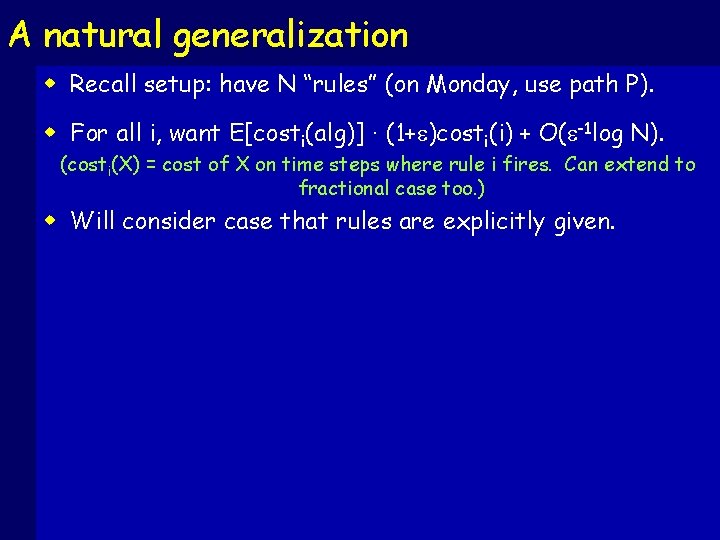
A natural generalization w Recall setup: have N “rules” (on Monday, use path P). w For all i, want E[costi(alg)] · (1+ )costi(i) + O( -1 log N). (costi(X) = cost of X on time steps where rule i fires. Can extend to fractional case too. ) w Will consider case that rules are explicitly given.

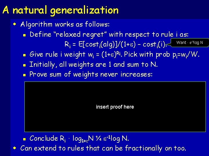
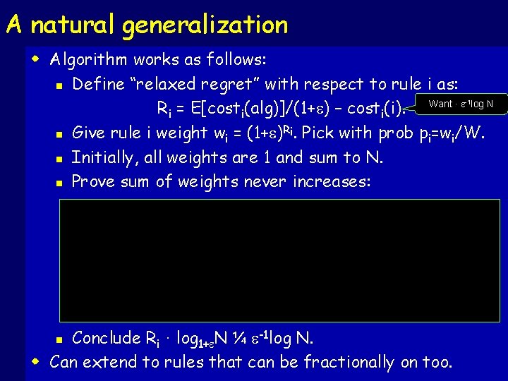
A natural generalization w Algorithm works as follows: n Define “relaxed regret” with respect to rule i as: Ri = E[costi(alg)]/(1+ ) – costi(i). Want · log N R n Give rule i weight wi = (1+ ) i. Pick with prob pi=wi/W. n Initially, all weights are 1 and sum to N. n Prove sum of weights never increases: -1 insert proof here Conclude Ri · log 1+ N ¼ -1 log N. w Can extend to rules that can be fractionally on too. n

A natural generalization w Algorithm works as follows: n Define “relaxed regret” with respect to rule i as: Ri = E[costi(alg)]/(1+ ) – costi(i). Want · log N R n Give rule i weight wi = (1+ ) i. Pick with prob pi=wi/W. n Initially, all weights are 1 and sum to N. n Prove sum of weights never increases: -1 Conclude Ri · log 1+ N ¼ -1 log N. w Can extend to rules that can be fractionally on too. n

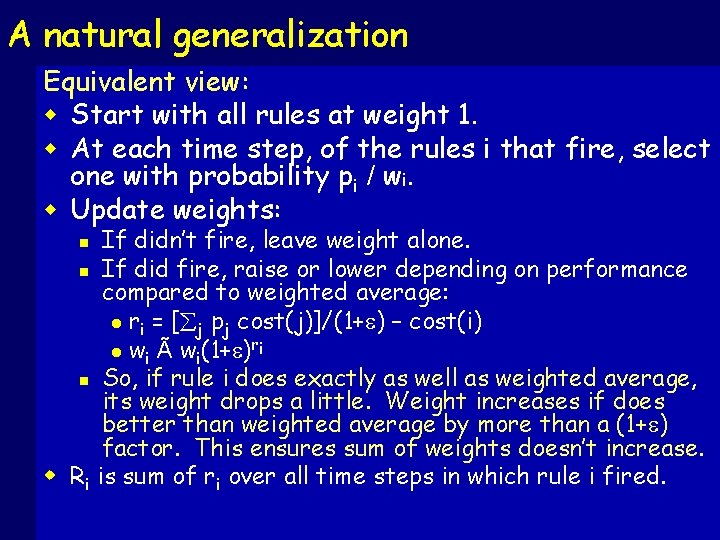
A natural generalization Equivalent view: w Start with all rules at weight 1. w At each time step, of the rules i that fire, select one with probability pi / wi. w Update weights: If didn’t fire, leave weight alone. n If did fire, raise or lower depending on performance compared to weighted average: l ri = [ j pj cost(j)]/(1+ ) – cost(i) l wi à wi(1+ )ri n So, if rule i does exactly as well as weighted average, its weight drops a little. Weight increases if does better than weighted average by more than a (1+ ) factor. This ensures sum of weights doesn’t increase. w Ri is sum of ri over all time steps in which rule i fired. n

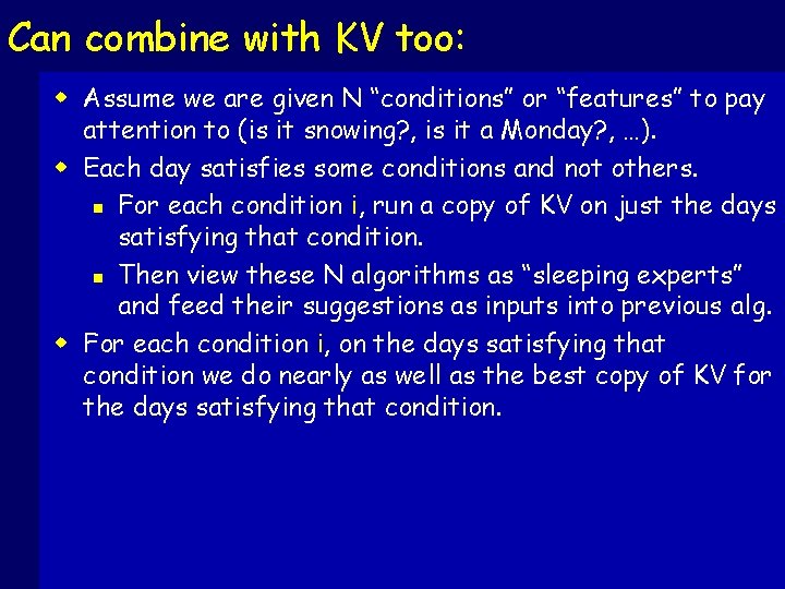
Can combine with KV too: w Assume we are given N “conditions” or “features” to pay attention to (is it snowing? , is it a Monday? , …). w Each day satisfies some conditions and not others. n For each condition i, run a copy of KV on just the days satisfying that condition. n Then view these N algorithms as “sleeping experts” and feed their suggestions as inputs into previous alg. w For each condition i, on the days satisfying that condition we do nearly as well as the best copy of KV for the days satisfying that condition.

Now to Part II…

What if everyone started using no-regret algs? w What if changing cost function is due to other players in the system optimizing for themselves? w No-regret can be viewed as a nice definition of reasonable self-interested behavior. So, what happens to overall system if everyone uses one? w In zero-sum games, behavior quickly approaches minimax optimal. w In general-sum games, does behavior quickly (or at all) approach a Nash equilibrium? (after all, a Nash Eq is exactly a set of distributions that are no-regret wrt each other). w Well, unfortunately, no.

A bad example for general-sum games w Augmented Shapley game from [Z 04]: “RPSF” n First 3 rows/cols are Shapley game (rock / paper / scissors but if both do same action then both lose). th action “play foosball” has slight negative if n 4 other player is still doing r/p/s but positive if other player does 4 th action too. n NR algs will cycle among first 3 and have no regret, but do worse than only Nash Equilibrium of both playing foosball. w We didn’t really expect this to work given how hard NE can be to find…

What can we say? w If algorithms minimize “internal” or “swap” regret, then empirical distribution of play approaches correlated equilibrium. n n n Foster & Vohra, Hart & Mas-Colell, … Alg joint with Yishay Mansour gives current best T as fn of size of game N. [don’t worry, I’ll define CE…] w In some natural cases, like routing in Wardrop model, can show daily traffic actually approaches Nash. n Work joint with Eyal Even-Dar and Katrina Ligett.

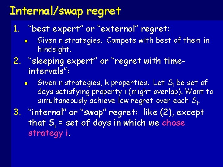
Internal/swap regret 1. “best expert” or “external” regret: n Given n strategies. Compete with best of them in hindsight. 2. “sleeping expert” or “regret with timeintervals”: n Given n strategies, k properties. Let Si be set of days satisfying property i (might overlap). Want to simultaneously achieve low regret over each Si. 3. “internal” or “swap” regret: like (2), except that Si = set of days in which we chose strategy i.

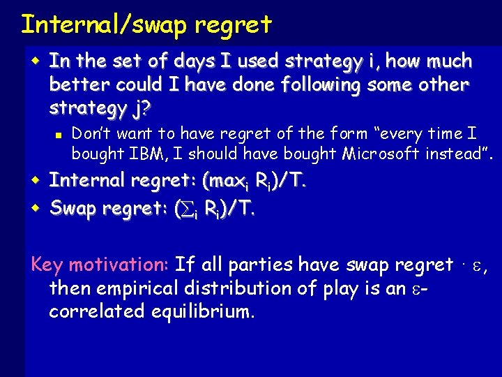
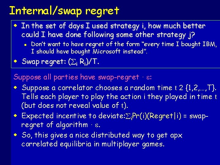
Internal/swap regret w In the set of days I used strategy i, how much better could I have done following some other strategy j? n w w Don’t want to have regret of the form “every time I bought IBM, I should have bought Microsoft instead”. Internal regret: (maxi Ri)/T. Swap regret: ( i Ri)/T. Key motivation: If all parties have swap regret · , then empirical distribution of play is an correlated equilibrium.

Internal/swap regret w In the set of days I used strategy i, how much better could I have done following some other strategy j? n Don’t want to have regret of the form “every time I bought IBM, I should have bought Microsoft instead”. w Swap regret: ( i Ri)/T. Suppose all parties have swap-regret · : w Suppose a correlator chooses a random time t 2 {1, 2, …, T}. Tells each player to play the action i they played in time t (but does not reveal value of t). w Expected incentive to deviate: i. Pr(i)(Regret|i) = swapregret of algorithm · . w So, this gives a nice distributed way to get apx correlated equilibria in multiplayer games.

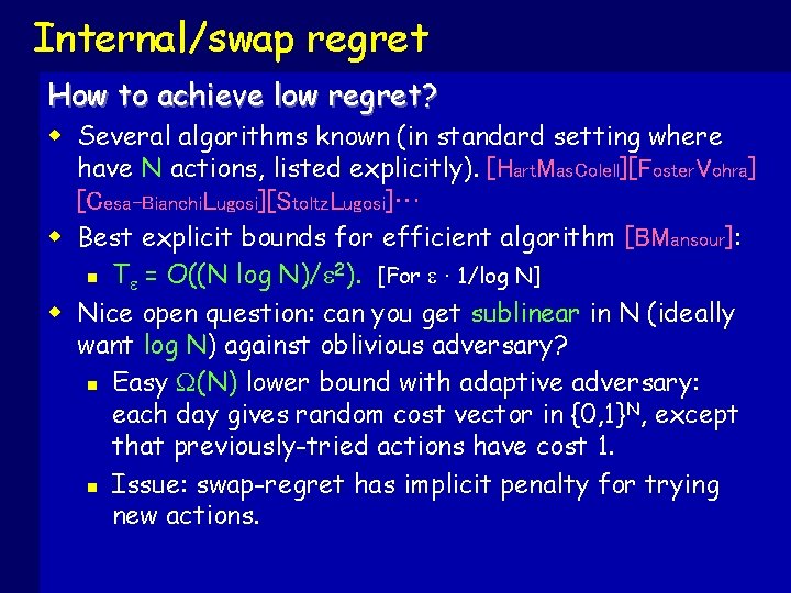
Internal/swap regret How to achieve low regret? w Several algorithms known (in standard setting where have N actions, listed explicitly). [Hart. Mas. Colell][Foster. Vohra] [Cesa-Bianchi. Lugosi][Stoltz. Lugosi]… w Best explicit bounds for efficient algorithm [BMansour]: 2 n T = O((N log N)/ ). [For · 1/log N] w Nice open question: can you get sublinear in N (ideally want log N) against oblivious adversary? n Easy (N) lower bound with adaptive adversary: each day gives random cost vector in {0, 1}N, except that previously-tried actions have cost 1. n Issue: swap-regret has implicit penalty for trying new actions.

[BMansour] algorithm: Plan: use a “best expert” algorithm A as subroutine. Idea: n Instantiate one copy Ai responsible for expected regret over times we play i. n If each Ai proposed to play qi, so all together we have matrix Q, then define p = p. Q. n Allows us to view pi as prob we chose action i or prob we chose algorithm Ai. n Each time step, if we play p=(p 1, …, pn) and get cost vector c=(c 1, …, cn), then Ai gets cost-vector pic. n Then do a few calculations to show this works. (but now)

Now on to the last part of the talk…

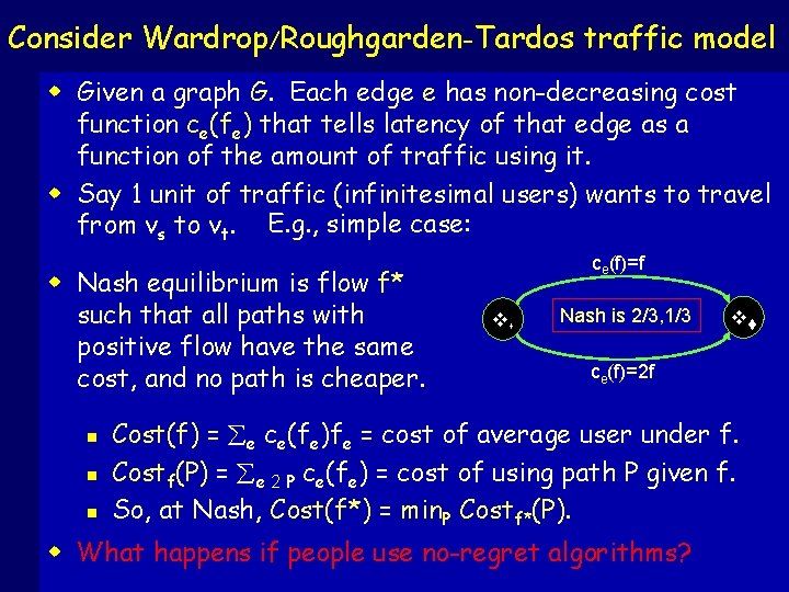
Consider Wardrop/Roughgarden-Tardos traffic model w Given a graph G. Each edge e has non-decreasing cost function ce(fe) that tells latency of that edge as a function of the amount of traffic using it. w Say 1 unit of traffic (infinitesimal users) wants to travel from vs to vt. E. g. , simple case: w Nash equilibrium is flow f* such that all paths with positive flow have the same cost, and no path is cheaper. n n n ce(f)=f vs Nash is 2/3, 1/3 vt ce(f)=2 f Cost(f) = e ce(fe)fe = cost of average user under f. Costf(P) = e 2 P ce(fe) = cost of using path P given f. So, at Nash, Cost(f*) = min. P Costf*(P). w What happens if people use no-regret algorithms?

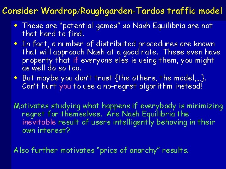
Consider Wardrop/Roughgarden-Tardos traffic model w These are “potential games” so Nash Equilibria are not that hard to find. w In fact, a number of distributed procedures are known that will approach Nash at a good rate. These even have property that if everyone else is using them, you might as well do so too. w But maybe you don’t trust {the others, the model, …}. Can’t hurt you to use a no-regret algorithm instead! Motivates studying what happens if everybody is minimizing regret for themselves. Are Nash Equilibria the inevitable result of users intelligently behaving in their own interest? Also further motivates “price of anarchy” results.

Global behavior of NR algs [B-Even. Dar-Ligett] On day t, have flow ft. Average regret by some time T. So, avgt[Cost(ft)] · + min. P avgt[Costft(P)]. What we’d like to say is the time-average flow favg is -Nash: Cost(favg) · + min. P Costfavg(P) w Or even better that most ft are -Nash: Cost(ft) · + min. P Costft(P) w But problems if cost functions are too sharp. w w 2/3 vs 1/3 vt

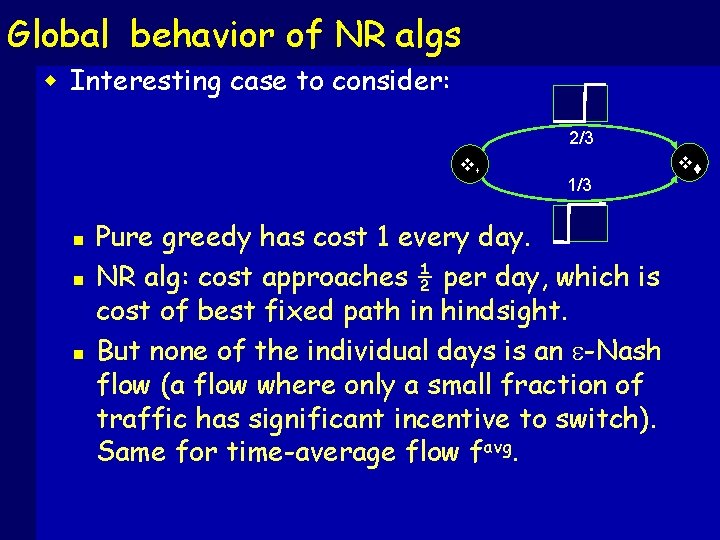
Global behavior of NR algs w Interesting case to consider: 2/3 vs n n n 1/3 Pure greedy has cost 1 every day. NR alg: cost approaches ½ per day, which is cost of best fixed path in hindsight. But none of the individual days is an -Nash flow (a flow where only a small fraction of traffic has significant incentive to switch). Same for time-average flow favg. vt

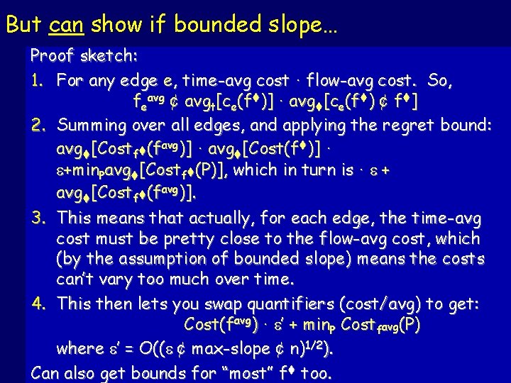
But can show if bounded slope… Proof sketch: 1. For any edge e, time-avg cost · flow-avg cost. So, feavg ¢ avgt[ce(ft)] · avgt[ce(ft) ¢ ft] 2. Summing over all edges, and applying the regret bound: avgt[Costft(favg)] · avgt[Cost(ft)] · +min. Pavgt[Costft(P)], which in turn is · + avgt[Costft(favg)]. 3. This means that actually, for each edge, the time- avg cost must be pretty close to the flow-avg cost, which (by the assumption of bounded slope) means the costs can’t vary too much over time. 4. This then lets you swap quantifiers (cost/avg) to get: Cost(favg) · ’ + min. P Costfavg(P) where ’ = O(( ¢ max-slope ¢ n)1/2). Can also get bounds for “most” ft too.

Some extensions w Can extend to multi-commodity case (different sources/destinations). w Can extend to case of different allowable subgraphs: n So each commodity is a (vs, vt, G’) triple. n For simple case of parallel links, this is “restricted machines setting”.

Summary/Open problems w Regret-minimizing algorithms esp motivated by online learning and routing-type problems. w “sleeping experts” algorithm can handle different Si. w Swap-regret related to correlated equilibria. w No-external-regret property sufficient to converge to Nash in Wardrop model. Open problems: w Time-bounds sublinear in N for achieving swap regret? w Other “price of minimizing regret / true-anarchy / adaptive self-interested behavior” results?