Neural Codes 1 Neuronal Codes Action potentials as

Neural Codes 1

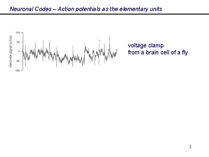
Neuronal Codes – Action potentials as the elementary units voltage clamp from a brain cell of a fly 2

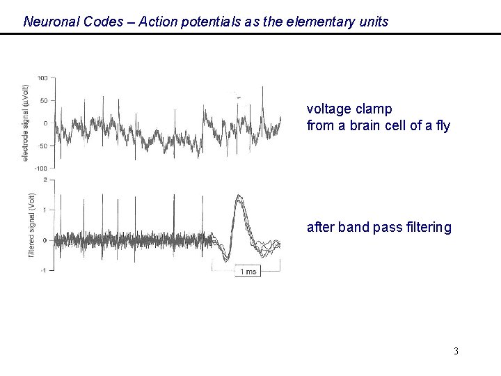
Neuronal Codes – Action potentials as the elementary units voltage clamp from a brain cell of a fly after band pass filtering 3

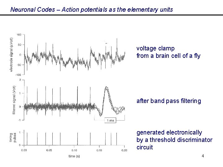
Neuronal Codes – Action potentials as the elementary units voltage clamp from a brain cell of a fly after band pass filtering generated electronically by a threshold discriminator circuit 4

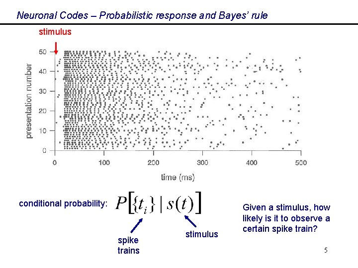
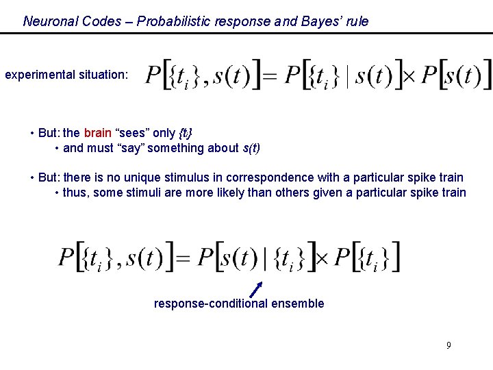
Neuronal Codes – Probabilistic response and Bayes’ rule stimulus conditional probability: spike trains stimulus Given a stimulus, how likely is it to observe a certain spike train? 5

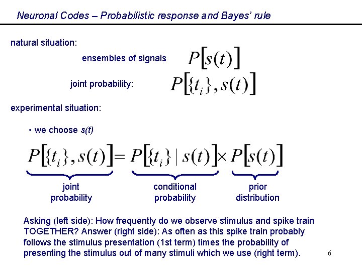
Neuronal Codes – Probabilistic response and Bayes’ rule natural situation: ensembles of signals joint probability: experimental situation: • we choose s(t) joint probability conditional probability prior distribution Asking (left side): How frequently do we observe stimulus and spike train TOGETHER? Answer (right side): As often as this spike train probably follows the stimulus presentation (1 st term) times the probability of presenting the stimulus out of many stimuli which we use (right term). 6

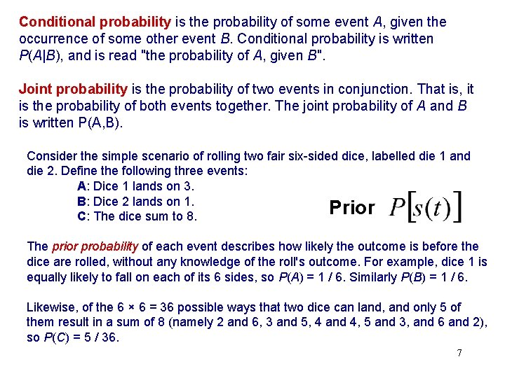
Conditional probability is the probability of some event A, given the occurrence of some other event B. Conditional probability is written P(A|B), and is read "the probability of A, given B". Joint probability is the probability of two events in conjunction. That is, it is the probability of both events together. The joint probability of A and B is written P(A, B). Consider the simple scenario of rolling two fair six-sided dice, labelled die 1 and die 2. Define the following three events: A: Dice 1 lands on 3. B: Dice 2 lands on 1. Prior C: The dice sum to 8. The prior probability of each event describes how likely the outcome is before the dice are rolled, without any knowledge of the roll's outcome. For example, dice 1 is equally likely to fall on each of its 6 sides, so P(A) = 1 / 6. Similarly P(B) = 1 / 6. Likewise, of the 6 × 6 = 36 possible ways that two dice can land, and only 5 of them result in a sum of 8 (namely 2 and 6, 3 and 5, 4 and 4, 5 and 3, and 6 and 2), so P(C) = 5 / 36. 7

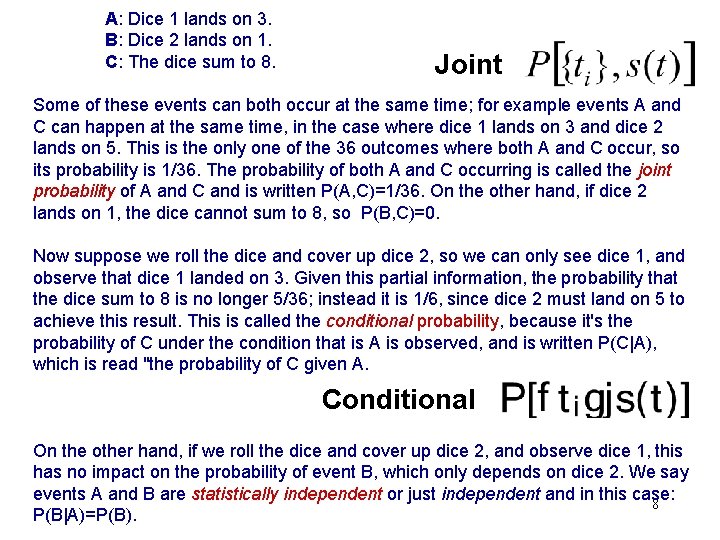
A: Dice 1 lands on 3. B: Dice 2 lands on 1. C: The dice sum to 8. Joint Some of these events can both occur at the same time; for example events A and C can happen at the same time, in the case where dice 1 lands on 3 and dice 2 lands on 5. This is the only one of the 36 outcomes where both A and C occur, so its probability is 1/36. The probability of both A and C occurring is called the joint probability of A and C and is written P(A, C)=1/36. On the other hand, if dice 2 lands on 1, the dice cannot sum to 8, so P(B, C)=0. Now suppose we roll the dice and cover up dice 2, so we can only see dice 1, and observe that dice 1 landed on 3. Given this partial information, the probability that the dice sum to 8 is no longer 5/36; instead it is 1/6, since dice 2 must land on 5 to achieve this result. This is called the conditional probability, because it's the probability of C under the condition that is A is observed, and is written P(C|A), which is read "the probability of C given A. Conditional On the other hand, if we roll the dice and cover up dice 2, and observe dice 1, this has no impact on the probability of event B, which only depends on dice 2. We say events A and B are statistically independent or just independent and in this case: 8 P(B|A)=P(B).

Neuronal Codes – Probabilistic response and Bayes’ rule experimental situation: • But: the brain “sees” only {ti} • and must “say” something about s(t) • But: there is no unique stimulus in correspondence with a particular spike train • thus, some stimuli are more likely than others given a particular spike train response-conditional ensemble 9

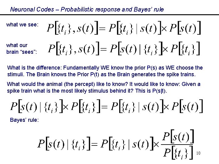
Neuronal Codes – Probabilistic response and Bayes’ rule what we see: what our brain “sees”: What is the difference: Fundamentally WE know the prior P(s) as WE choose the stimuli. The Brain knows the Prior P(t) as the Brain generates the spike trains. What would the animal (the percept) like to know? It would like to know: Given a spike train what is the most likely stimulus behind it? This is P(s|t). Bayes’ rule: 10

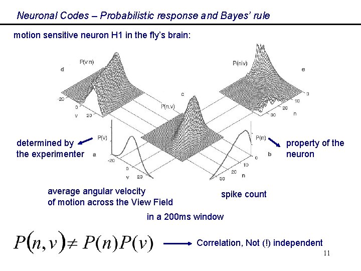
Neuronal Codes – Probabilistic response and Bayes’ rule motion sensitive neuron H 1 in the fly’s brain: determined by the experimenter property of the neuron average angular velocity of motion across the View Field spike count in a 200 ms window Correlation, Not (!) independent 11

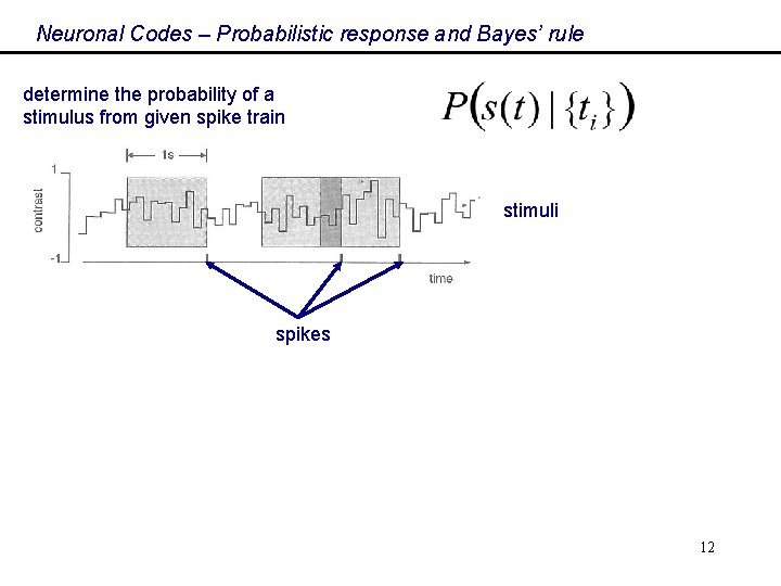
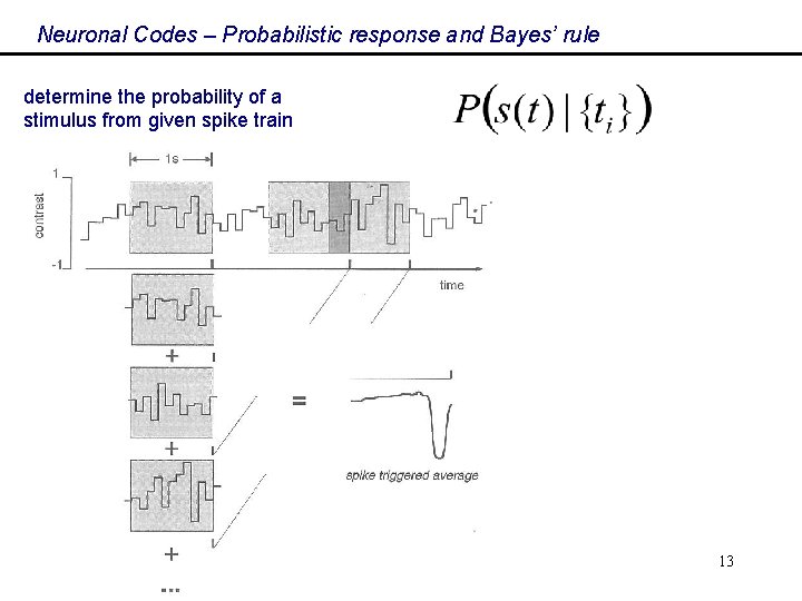
Neuronal Codes – Probabilistic response and Bayes’ rule determine the probability of a stimulus from given spike train stimuli spikes 12

Neuronal Codes – Probabilistic response and Bayes’ rule determine the probability of a stimulus from given spike train 13

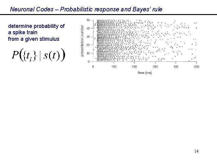
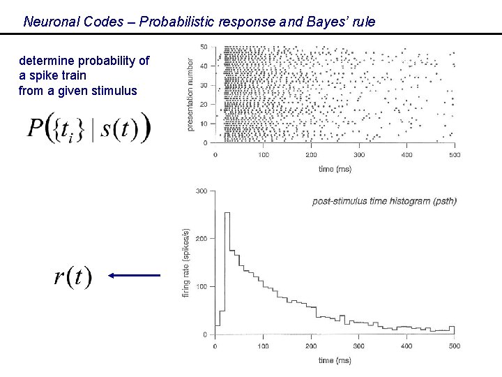
Neuronal Codes – Probabilistic response and Bayes’ rule determine probability of a spike train from a given stimulus 14

Neuronal Codes – Probabilistic response and Bayes’ rule determine probability of a spike train from a given stimulus 15

Neuronal Codes – Probabilistic response and Bayes’ rule Nice probabilistic stuff, but SO, WHAT? 17

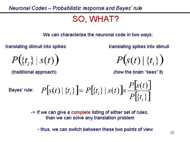
Neuronal Codes – Probabilistic response and Bayes’ rule SO, WHAT? We can characterize the neuronal code in two ways: translating stimuli into spikes (traditional approach) translating spikes into stimuli (how the brain “sees” it) Bayes’ rule: -> If we can give a complete listing of either set of rules, than we can solve any translation problem • thus, we can switch between these two points of view 18

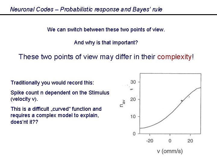
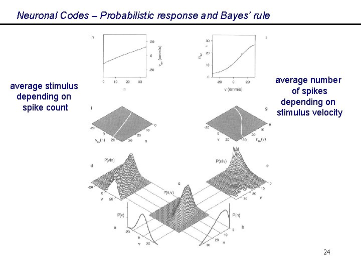
Neuronal Codes – Probabilistic response and Bayes’ rule We can switch between these two points of view. And why is that important? These two points of view may differ in their complexity! Traditionally you would record this: Spike count n dependent on the Stimulus (velocity v). This is a difficult „curved“ function and requires a complex model to explain, does‘nt it? ? 20

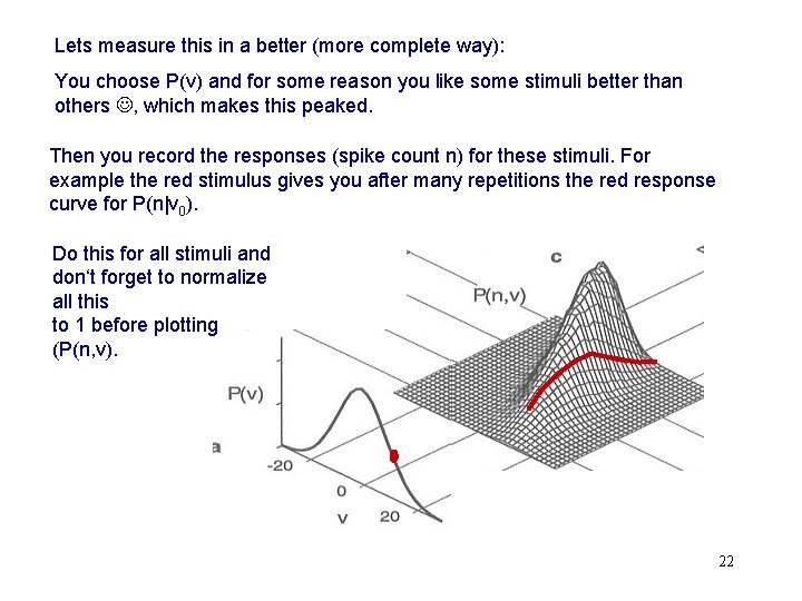
Lets measure this in a better (more complete way): You choose P(v) and for some reason you like some stimuli better than others , which makes this peaked. Then you record the responses (spike count n) for these stimuli. For example the red stimulus gives you after many repetitions the red response curve for P(n|v 0). Do this for all stimuli and don‘t forget to normalize all this to 1 before plotting (P(n, v). 22

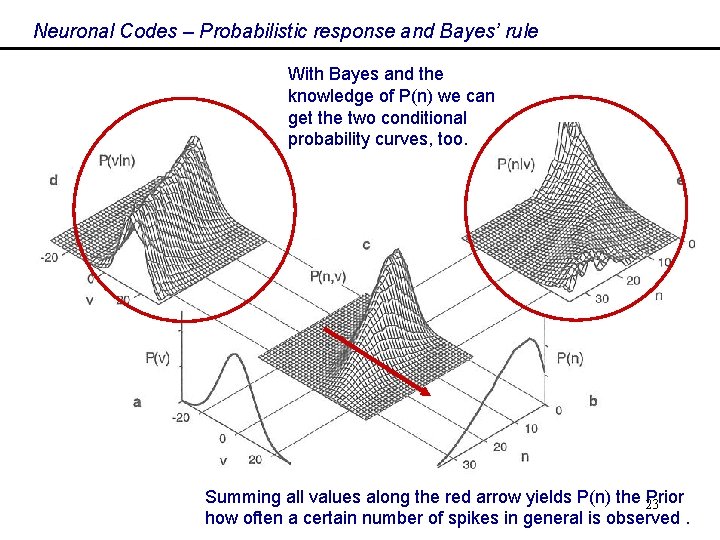
Neuronal Codes – Probabilistic response and Bayes’ rule With Bayes and the knowledge of P(n) we can get the two conditional probability curves, too. Summing all values along the red arrow yields P(n) the 23 Prior how often a certain number of spikes in general is observed.

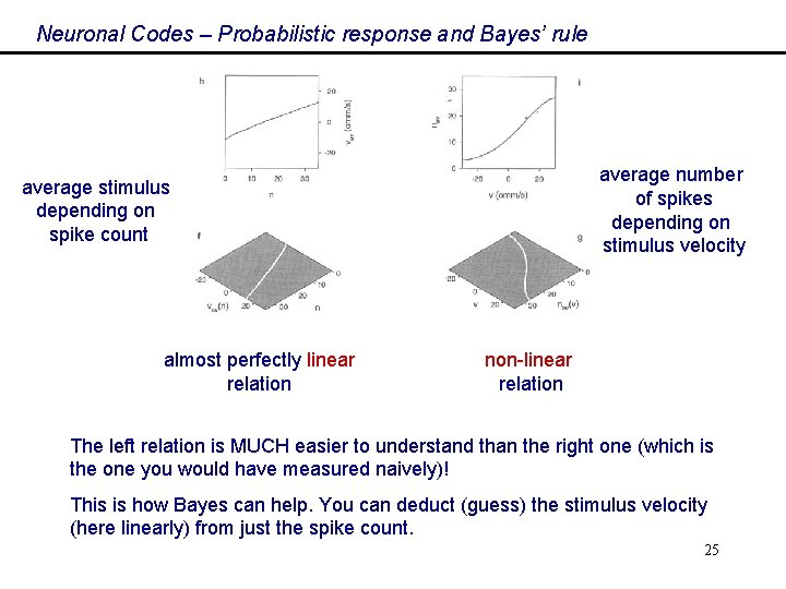
Neuronal Codes – Probabilistic response and Bayes’ rule average stimulus depending on spike count average number of spikes depending on stimulus velocity 24

Neuronal Codes – Probabilistic response and Bayes’ rule average number of spikes depending on stimulus velocity average stimulus depending on spike count almost perfectly linear relation non-linear relation The left relation is MUCH easier to understand than the right one (which is the one you would have measured naively)! This is how Bayes can help. You can deduct (guess) the stimulus velocity (here linearly) from just the spike count. 25

Neuronal Codes – Probabilistic response and Bayes’ rule For a deeper discussion read, for instance, that nice, difficult book: Rieke, F. et al. (1996). Spikes: Exploring the neural code. MIT Press. 26