MultiEchelon Inventory Management Prof Larry Snyder Lehigh University

Multi-Echelon Inventory Management Prof. Larry Snyder Lehigh University Dept. of Industrial & Systems Engineering OR Roundtable, June 15, 2006

Outline n Introduction q q n n Overview Network topology Assumptions Deterministic models Stochastic models Decentralized systems Multi-Echelon Inventory – June 15, 2006

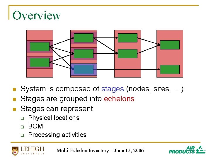
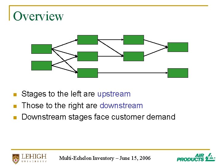
Overview n n n System is composed of stages (nodes, sites, …) Stages are grouped into echelons Stages can represent q q q Physical locations BOM Processing activities Multi-Echelon Inventory – June 15, 2006

Overview n n n Stages to the left are upstream Those to the right are downstream Downstream stages face customer demand Multi-Echelon Inventory – June 15, 2006

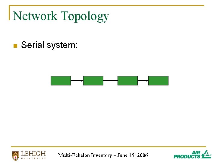
Network Topology n Serial system: Multi-Echelon Inventory – June 15, 2006

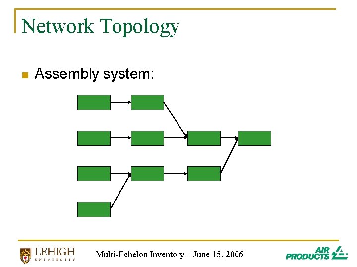
Network Topology n Assembly system: Multi-Echelon Inventory – June 15, 2006

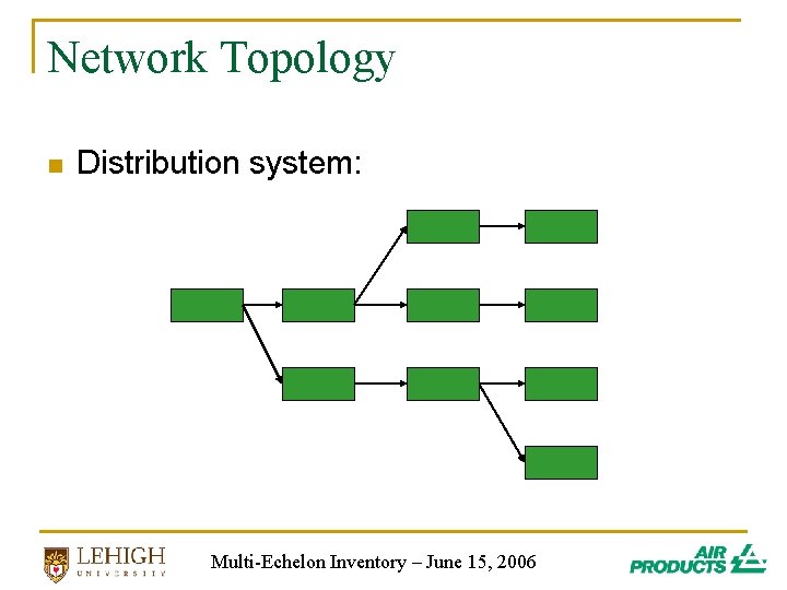
Network Topology n Distribution system: Multi-Echelon Inventory – June 15, 2006

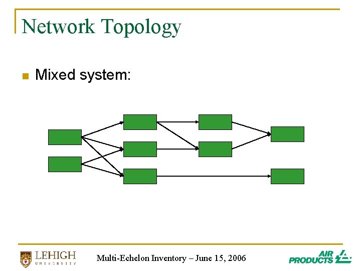
Network Topology n Mixed system: Multi-Echelon Inventory – June 15, 2006

Assumptions n Periodic review q n Centralized decision making q q n Period = week, month, … Can optimize system globally Later, I will talk about decentralized systems Costs q q q Holding cost Fixed order cost Stockout cost (vs. service level) Multi-Echelon Inventory – June 15, 2006

Deterministic Models n Suppose everything in the system is deterministic (not random) q q n n Demands, lead times, … Possible to achieve 100% service If no fixed costs, explode BOM every period If fixed costs are non-negligible, key tradeoff is between fixed and holding costs q q Multi-echelon version of EOQ MRP systems (optimization component) Multi-Echelon Inventory – June 15, 2006

Outline n n Introduction Stochastic models q q n Base-stock model Stochastic multi-echelon systems Strategic safety stock placement Supply uncertainty Decentralized systems Multi-Echelon Inventory – June 15, 2006

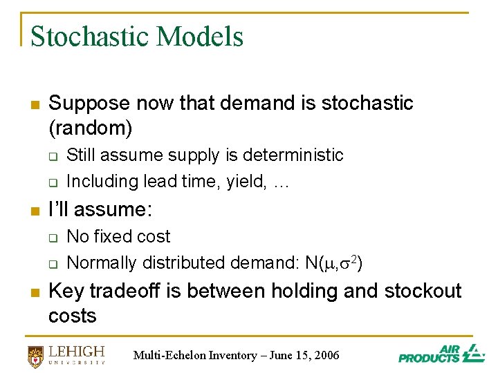
Stochastic Models n Suppose now that demand is stochastic (random) q q n I’ll assume: q q n Still assume supply is deterministic Including lead time, yield, … No fixed cost Normally distributed demand: N( , 2) Key tradeoff is between holding and stockout costs Multi-Echelon Inventory – June 15, 2006

The Base-Stock Model n n Single stage (and echelon) Excess inventory incurs holding cost of h per unit period Unmet demand is backordered at a cost of p per unit period Stage follows base-stock policy q q q Each period, “order up to” base-stock level, y aka order-up-to policy Similar to days-of-supply policy: y / DOS Multi-Echelon Inventory – June 15, 2006

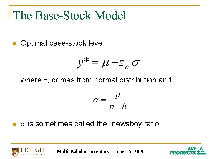
The Base-Stock Model n Optimal base-stock level: where z comes from normal distribution and n is sometimes called the “newsboy ratio” Multi-Echelon Inventory – June 15, 2006

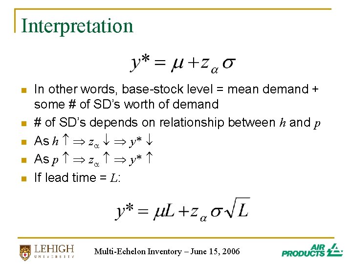
Interpretation n n In other words, base-stock level = mean demand + some # of SD’s worth of demand # of SD’s depends on relationship between h and p As h z y* As p z y* If lead time = L: Multi-Echelon Inventory – June 15, 2006

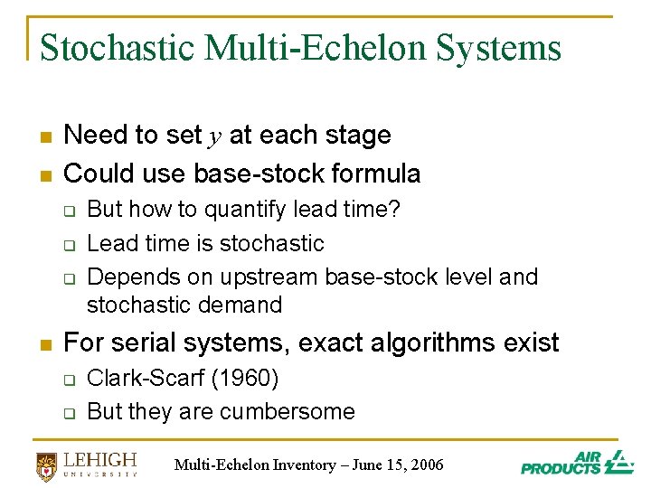
Stochastic Multi-Echelon Systems n n Need to set y at each stage Could use base-stock formula q q q n But how to quantify lead time? Lead time is stochastic Depends on upstream base-stock level and stochastic demand For serial systems, exact algorithms exist q q Clark-Scarf (1960) But they are cumbersome Multi-Echelon Inventory – June 15, 2006

An Approximate Method n Assume that each stage carries sufficient inventory to deliver product within S periods “most of the time” q q n Definition of “most” depends on service level constant, z S is called the committed service time (CST) We simply ignore the times that the stage does not meet its CST q q For the purposes of the optimization Allows us to pretend LT is deterministic Multi-Echelon Inventory – June 15, 2006

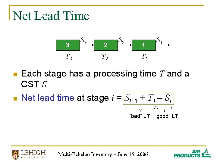
Net Lead Time 3 T 3 n n S 3 2 T 2 S 2 1 S 1 T 1 Each stage has a processing time T and a CST S Net lead time at stage i = Si+1 + Ti – Si “bad” LT “good” LT Multi-Echelon Inventory – June 15, 2006

Net Lead Time vs. Inventory n Suppose Si = Si+1 + Ti q q q n e. g. , inbound CST = 4, proc time = 2, outbound CST = 6 Don’t need to hold any inventory Operate entirely as pull (make-to-order, JIT) system Suppose Si = 0 q q Promise immediate order fulfillment Make-to-stock system Multi-Echelon Inventory – June 15, 2006

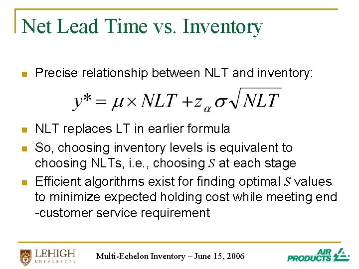
Net Lead Time vs. Inventory n Precise relationship between NLT and inventory: n NLT replaces LT in earlier formula So, choosing inventory levels is equivalent to choosing NLTs, i. e. , choosing S at each stage Efficient algorithms exist for finding optimal S values to minimize expected holding cost while meeting end -customer service requirement n n Multi-Echelon Inventory – June 15, 2006

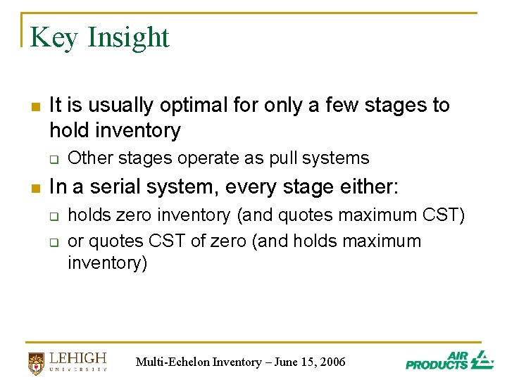
Key Insight n It is usually optimal for only a few stages to hold inventory q n Other stages operate as pull systems In a serial system, every stage either: q q holds zero inventory (and quotes maximum CST) or quotes CST of zero (and holds maximum inventory) Multi-Echelon Inventory – June 15, 2006

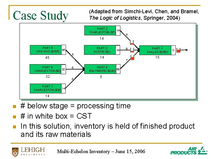
Case Study (Adapted from Simchi-Levi, Chen, and Bramel, The Logic of Logistics, Springer, 2004) PART 2 14 CHARLESTON ($7) 8 14 PART 5 45 CHICAGO ($155) 45 PART 6 32 CHARLESTON ($2) 32 5 8 8 PART 3 AUSTIN ($2) 14 14 6 7 PART 1 DALLAS ($260) 0 15 PART 4 55 BALTIMORE ($220) 5 PART 7 14 CHARLESTON ($30) 14 n n n # below stage = processing time # in white box = CST In this solution, inventory is held of finished product and its raw materials Multi-Echelon Inventory – June 15, 2006

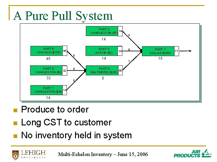
A Pure Pull System PART 2 14 CHARLESTON ($7) 8 14 PART 5 45 CHICAGO ($155) 45 PART 6 32 CHARLESTON ($2) 32 5 8 8 PART 3 AUSTIN ($2) 14 14 6 7 PART 4 55 BALTIMORE ($220) 5 PART 7 14 CHARLESTON ($30) 14 n n n Produce to order Long CST to customer No inventory held in system Multi-Echelon Inventory – June 15, 2006 PART 1 DALLAS ($260) 15 77

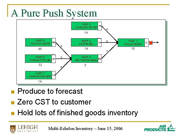
A Pure Push System PART 2 14 CHARLESTON ($7) 8 14 PART 5 45 CHICAGO ($155) 45 PART 6 32 CHARLESTON ($2) 32 5 8 8 PART 3 AUSTIN ($2) 14 14 6 7 PART 1 DALLAS ($260) 15 PART 4 55 BALTIMORE ($220) 5 PART 7 14 CHARLESTON ($30) 14 n n n Produce to forecast Zero CST to customer Hold lots of finished goods inventory Multi-Echelon Inventory – June 15, 2006 0

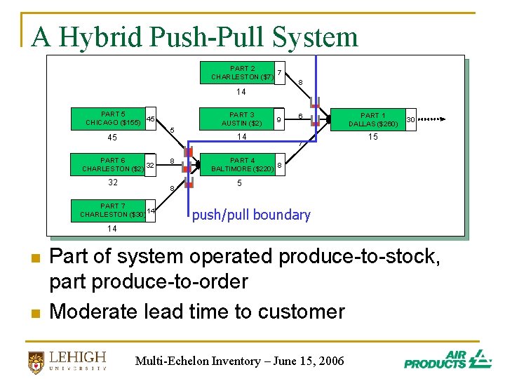
A Hybrid Push-Pull System PART 2 7 CHARLESTON ($7) 8 14 PART 5 45 CHICAGO ($155) 45 PART 6 32 CHARLESTON ($2) 32 5 8 8 PART 7 14 CHARLESTON ($30) PART 3 AUSTIN ($2) 9 14 6 7 PART 1 DALLAS ($260) 30 15 PART 4 8 BALTIMORE ($220) 5 push/pull boundary 14 n n Part of system operated produce-to-stock, part produce-to-order Moderate lead time to customer Multi-Echelon Inventory – June 15, 2006

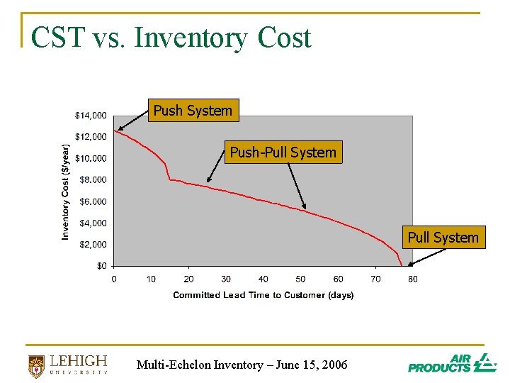
CST vs. Inventory Cost Push System Push-Pull System Multi-Echelon Inventory – June 15, 2006

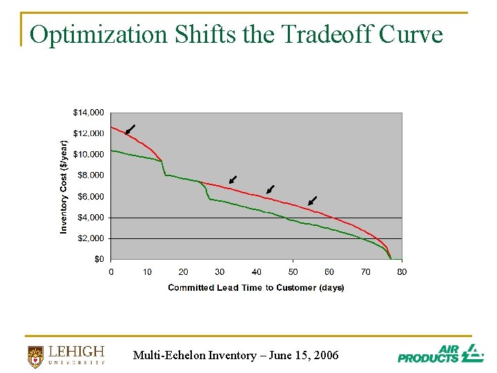
Optimization Shifts the Tradeoff Curve Multi-Echelon Inventory – June 15, 2006

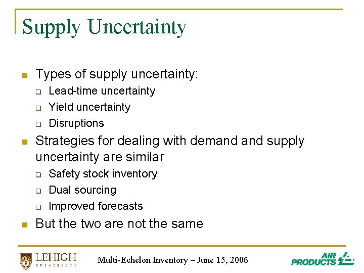
Supply Uncertainty n Types of supply uncertainty: q q q n Strategies for dealing with demand supply uncertainty are similar q q q n Lead-time uncertainty Yield uncertainty Disruptions Safety stock inventory Dual sourcing Improved forecasts But the two are not the same Multi-Echelon Inventory – June 15, 2006

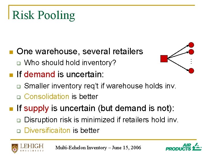
Risk Pooling n One warehouse, several retailers n If demand is uncertain: q q n Who should hold inventory? Smaller inventory req’t if warehouse holds inv. Consolidation is better If supply is uncertain (but demand is not): q q Disruption risk is minimized if retailers hold inv. Diversificaiton is better Multi-Echelon Inventory – June 15, 2006 … q

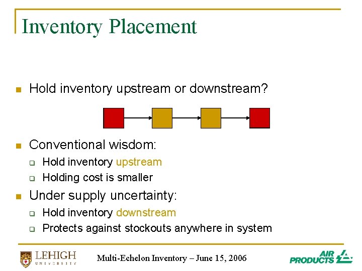
Inventory Placement n Hold inventory upstream or downstream? n Conventional wisdom: q q n Hold inventory upstream Holding cost is smaller Under supply uncertainty: q q Hold inventory downstream Protects against stockouts anywhere in system Multi-Echelon Inventory – June 15, 2006

Outline n n n Introduction Stochastic models Decentralized systems q q q Suboptimality Contracting The bullwhip effect Multi-Echelon Inventory – June 15, 2006

Decentralized Systems n So far, we have assumed the system is centralized q q n Can optimize at all stages globally One stage may incur higher costs to benefit the system as a whole What if each stage acts independently to minimize its own cost / maximize its own profit? Multi-Echelon Inventory – June 15, 2006

Suboptimality n n Optimizing locally is likely to result in some degree of suboptimality Example: upstream stages want to operate make-to-order q n Results in too much inventory downstream Another example: q q q Wholesaler chooses wholesale price Retailer chooses order quantity Optimizing independently, the two parties will always leave money on the table Multi-Echelon Inventory – June 15, 2006

Contracting n One solution is for the parties to impose a contracting mechanism q q q n Splits the costs / profits / risks / rewards Still allows each party to act in its own best interest If structured correctly, system achieves optimal cost / profit, even with parties acting selfishly There is a large body of literature on contracting q q In practice, idea is commonly used Actual OR models rarely implemented Multi-Echelon Inventory – June 15, 2006

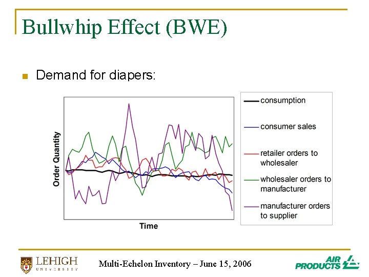
Bullwhip Effect (BWE) n Demand for diapers: Multi-Echelon Inventory – June 15, 2006

Irrational Behavior Causes BWE n Firms over-react to demand signals q q n n n Order too much when they perceive an upward demand trend Then back off when they accumulate too much inventory Firms under-weight the supply line Both are irrational behaviors Demonstrated by “beer game” Multi-Echelon Inventory – June 15, 2006

Rational Behavior Causes BWE n n Famous paper by Hau Lee, et al. (1997) BWE can be cause by rational behavior q n i. e. , by acting in “optimal” ways according to OR inventory models Four causes: q q Demand forecast updating Batch ordering Rationing game Price variations Multi-Echelon Inventory – June 15, 2006

Questions?