Walter Nicholson Amherst College Christopher Snyder Dartmouth College

Walter Nicholson Amherst College Christopher Snyder Dartmouth College Power. Point Slide Presentation | Philip Heap, James Madison University © 2015 Cengage Learning. All Rights Reserved. May not be scanned, copied or duplicated, or posted to a publicly accessible website, in whole or in part. 1

CHAPTER 6 Production © 2015 Cengage Learning. All Rights Reserved. May not be scanned, copied or duplicated, or posted to a publicly accessible website, in whole or in part. 2

Chapter Preview • We now want to turn to firm behavior, and answer three main questions. 1. What happens to output as a firm increases the number of input(s) it uses? 2. To what degree is a firm able to substitute one input for another? 3. What happens to production as a result of technological change? © 2015 Cengage Learning. All Rights Reserved. May not be scanned, copied or duplicated, or posted to a publicly accessible website, in whole or in part. Ch. 6 • 3

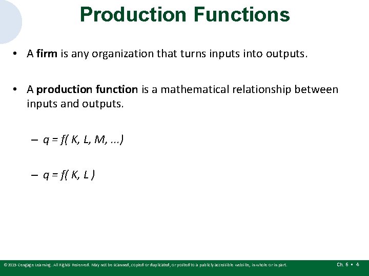
Production Functions • A firm is any organization that turns inputs into outputs. • A production function is a mathematical relationship between inputs and outputs. – q = f( K, L, M, . . . ) – q = f( K, L ) © 2015 Cengage Learning. All Rights Reserved. May not be scanned, copied or duplicated, or posted to a publicly accessible website, in whole or in part. Ch. 6 • 4

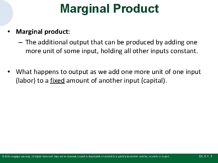
Marginal Product • Marginal product: – The additional output that can be produced by adding one more unit of some input, holding all other inputs constant. • What happens to output as we add one more unit of one input (labor) to a fixed amount of another input (capital). © 2015 Cengage Learning. All Rights Reserved. May not be scanned, copied or duplicated, or posted to a publicly accessible website, in whole or in part. Ch. 6 • 5

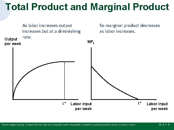
Total Product and Marginal Product Output per week As labor increases output increases but at a diminishing rate. So marginal product decreases as labor increases. MPL L* Labor input per week © 2015 Cengage Learning. All Rights Reserved. May not be scanned, copied or duplicated, or posted to a publicly accessible website, in whole or in part. L* Labor input per week Ch. 6 • 6

Average Product • Average product is equal to total output divided by the number of workers. • Average product tells you how productive all your workers are on average. It does not tell you how productive an extra worker is. • Practical difficulty in applying the marginal product concept. © 2015 Cengage Learning. All Rights Reserved. May not be scanned, copied or duplicated, or posted to a publicly accessible website, in whole or in part. Ch. 6 • 7

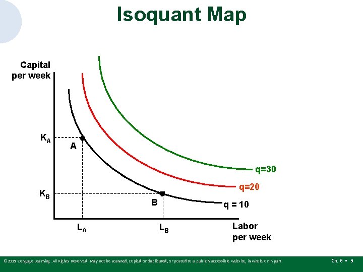
Isoquant Maps • How can a firm combine different amounts of capital and labor to produce output? • Isoquant: – A curve that shows the various combinations of inputs that will produce the same (a particular) amount of output. – How does this compare to an indifference curve? • Isoquant map is a contour map of a firm’s production function. © 2015 Cengage Learning. All Rights Reserved. May not be scanned, copied or duplicated, or posted to a publicly accessible website, in whole or in part. Ch. 6 • 8

Isoquant Map Capital per week KA A q=30 q=20 KB B LA q = 10 LB Labor per week © 2015 Cengage Learning. All Rights Reserved. May not be scanned, copied or duplicated, or posted to a publicly accessible website, in whole or in part. Ch. 6 • 9

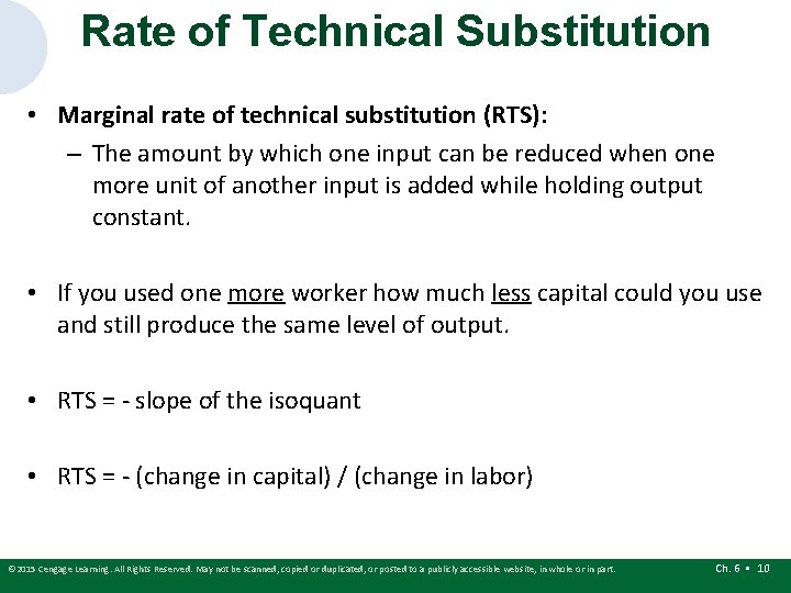
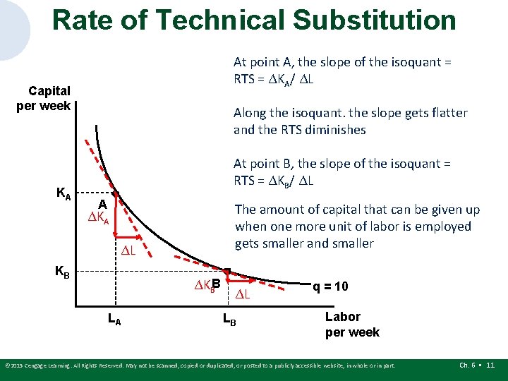
Rate of Technical Substitution • Marginal rate of technical substitution (RTS): – The amount by which one input can be reduced when one more unit of another input is added while holding output constant. • If you used one more worker how much less capital could you use and still produce the same level of output. • RTS = - slope of the isoquant • RTS = - (change in capital) / (change in labor) © 2015 Cengage Learning. All Rights Reserved. May not be scanned, copied or duplicated, or posted to a publicly accessible website, in whole or in part. Ch. 6 • 10

Rate of Technical Substitution At point A, the slope of the isoquant = RTS = ΔKA/ ΔL Capital per week KA Along the isoquant. the slope gets flatter and the RTS diminishes At point B, the slope of the isoquant = RTS = ΔKB/ ΔL A The amount of capital that can be given up when one more unit of labor is employed gets smaller and smaller ΔKA ΔL KB ΔKBB LA ΔL LB q = 10 Labor per week © 2015 Cengage Learning. All Rights Reserved. May not be scanned, copied or duplicated, or posted to a publicly accessible website, in whole or in part. Ch. 6 • 11

The RTS and Marginal Product • Why must the slope of the isoquant be negative or the RTS positive? – RTS = MPL/MPK – If RTS was < 0 either MPL or the MPK would also have to be < 0. – But then a firm would be paying for an input that reduced output. – Since no firm would do that MP’s > 0 and the RTS > 0. © 2015 Cengage Learning. All Rights Reserved. May not be scanned, copied or duplicated, or posted to a publicly accessible website, in whole or in part. Ch. 6 • 12

The RTS and Marginal Product • Why does the slope of the isoquant get flatter or why does the RTS diminish? – The less (more) labor is used relative to capital, the more (less) able labor is able to replace capital in production. – As the firm uses more and more labor, the MPL falls. – Therefore, to maintain the same level of output, the firm would only be able to give up smaller and smaller amounts of capital. © 2015 Cengage Learning. All Rights Reserved. May not be scanned, copied or duplicated, or posted to a publicly accessible website, in whole or in part. Ch. 6 • 13

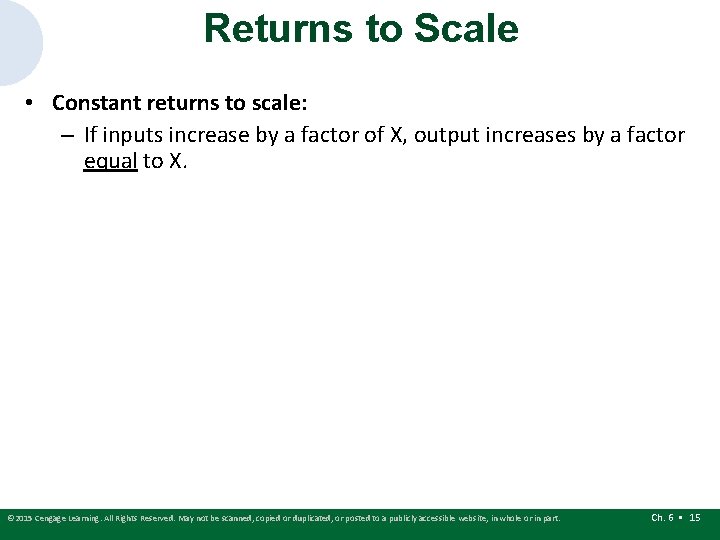
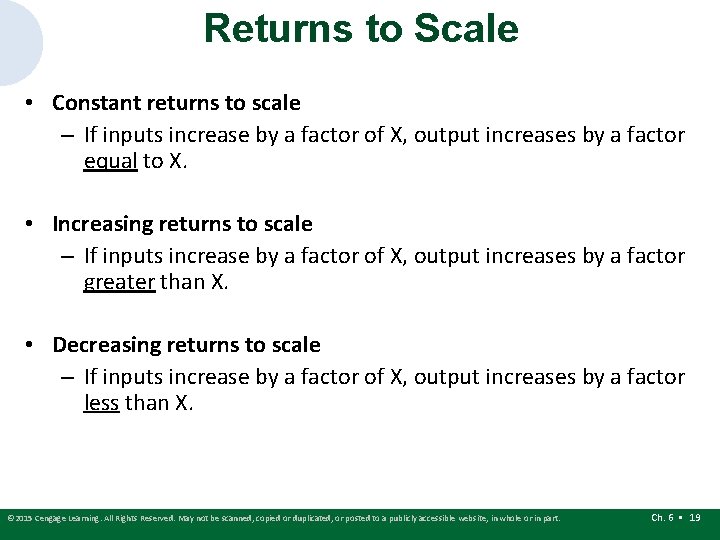
Returns to Scale • What would happen to production if a firm increased the number of all inputs? • Returns to scale: – The rate at which output increases in response to a proportional increases in all inputs. • Two opposing effects at work as scale increases: – Greater division of labor (specialization). – Managerial inefficiencies and coordination problems © 2015 Cengage Learning. All Rights Reserved. May not be scanned, copied or duplicated, or posted to a publicly accessible website, in whole or in part. Ch. 6 • 14

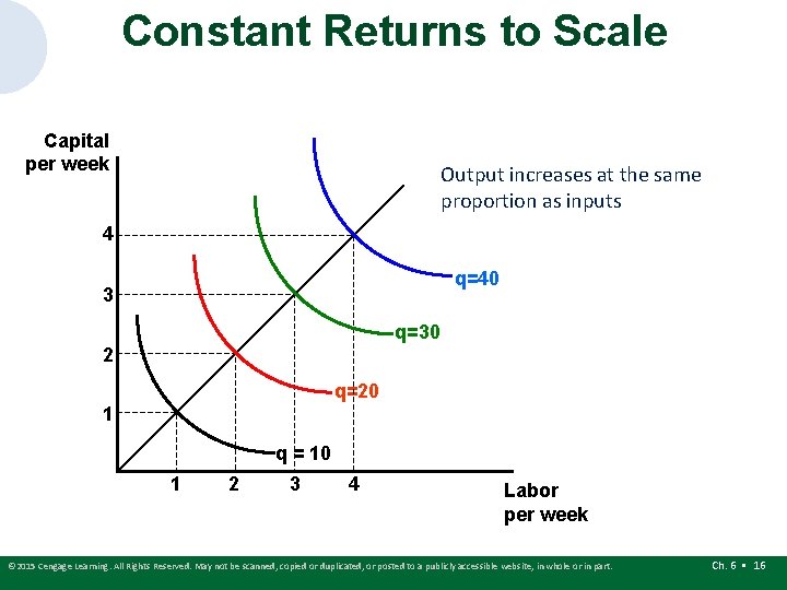
Returns to Scale • Constant returns to scale: – If inputs increase by a factor of X, output increases by a factor equal to X. © 2015 Cengage Learning. All Rights Reserved. May not be scanned, copied or duplicated, or posted to a publicly accessible website, in whole or in part. Ch. 6 • 15

Constant Returns to Scale Capital per week Output increases at the same proportion as inputs 4 q=40 3 q=30 2 q=20 1 q = 10 1 2 3 4 Labor per week © 2015 Cengage Learning. All Rights Reserved. May not be scanned, copied or duplicated, or posted to a publicly accessible website, in whole or in part. Ch. 6 • 16

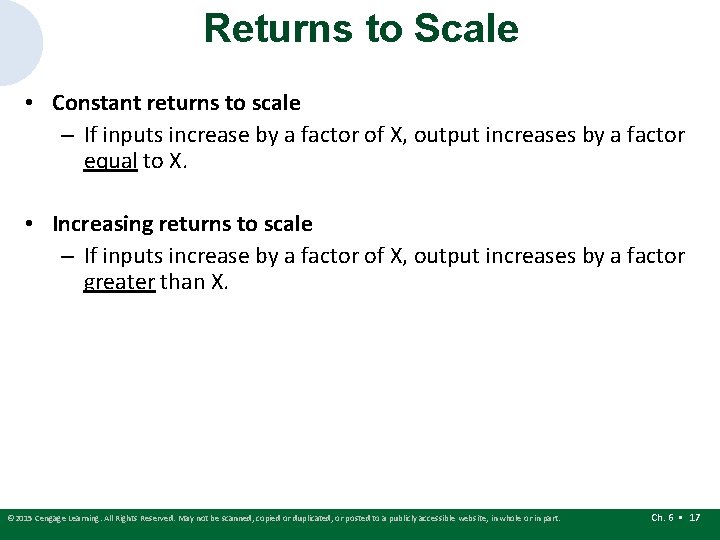
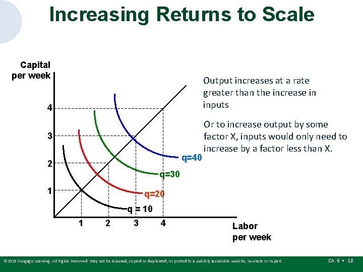
Returns to Scale • Constant returns to scale – If inputs increase by a factor of X, output increases by a factor equal to X. • Increasing returns to scale – If inputs increase by a factor of X, output increases by a factor greater than X. © 2015 Cengage Learning. All Rights Reserved. May not be scanned, copied or duplicated, or posted to a publicly accessible website, in whole or in part. Ch. 6 • 17

Increasing Returns to Scale Capital per week Output increases at a rate greater than the increase in inputs 4 3 q=40 2 Or to increase output by some factor X, inputs would only need to increase by a factor less than X. q=30 1 q=20 q = 10 1 2 3 4 Labor per week © 2015 Cengage Learning. All Rights Reserved. May not be scanned, copied or duplicated, or posted to a publicly accessible website, in whole or in part. Ch. 6 • 18

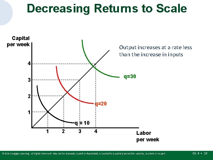
Returns to Scale • Constant returns to scale – If inputs increase by a factor of X, output increases by a factor equal to X. • Increasing returns to scale – If inputs increase by a factor of X, output increases by a factor greater than X. • Decreasing returns to scale – If inputs increase by a factor of X, output increases by a factor less than X. © 2015 Cengage Learning. All Rights Reserved. May not be scanned, copied or duplicated, or posted to a publicly accessible website, in whole or in part. Ch. 6 • 19

Decreasing Returns to Scale Capital per week Output increases at a rate less than the increase in inputs 4 q=30 3 2 q=20 1 q = 10 1 2 3 4 Labor per week © 2015 Cengage Learning. All Rights Reserved. May not be scanned, copied or duplicated, or posted to a publicly accessible website, in whole or in part. Ch. 6 • 20

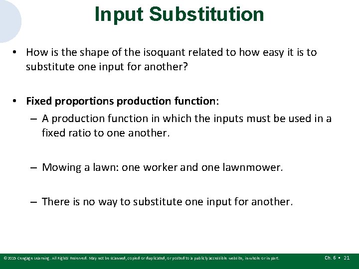
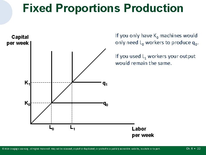
Input Substitution • How is the shape of the isoquant related to how easy it is to substitute one input for another? • Fixed proportions production function: – A production function in which the inputs must be used in a fixed ratio to one another. – Mowing a lawn: one worker and one lawnmower. – There is no way to substitute one input for another. © 2015 Cengage Learning. All Rights Reserved. May not be scanned, copied or duplicated, or posted to a publicly accessible website, in whole or in part. Ch. 6 • 21

Fixed Proportions Production If you only have K 0 machines would only need L 0 workers to produce q 0. Capital per week If you used L 1 workers your output would remain the same. K 1 q 1 K 0 q 0 L 1 Labor per week © 2015 Cengage Learning. All Rights Reserved. May not be scanned, copied or duplicated, or posted to a publicly accessible website, in whole or in part. Ch. 6 • 22

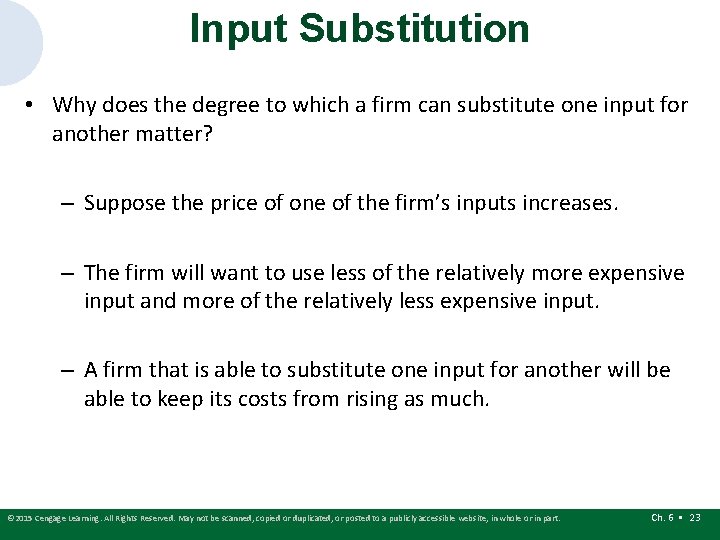
Input Substitution • Why does the degree to which a firm can substitute one input for another matter? – Suppose the price of one of the firm’s inputs increases. – The firm will want to use less of the relatively more expensive input and more of the relatively less expensive input. – A firm that is able to substitute one input for another will be able to keep its costs from rising as much. © 2015 Cengage Learning. All Rights Reserved. May not be scanned, copied or duplicated, or posted to a publicly accessible website, in whole or in part. Ch. 6 • 23

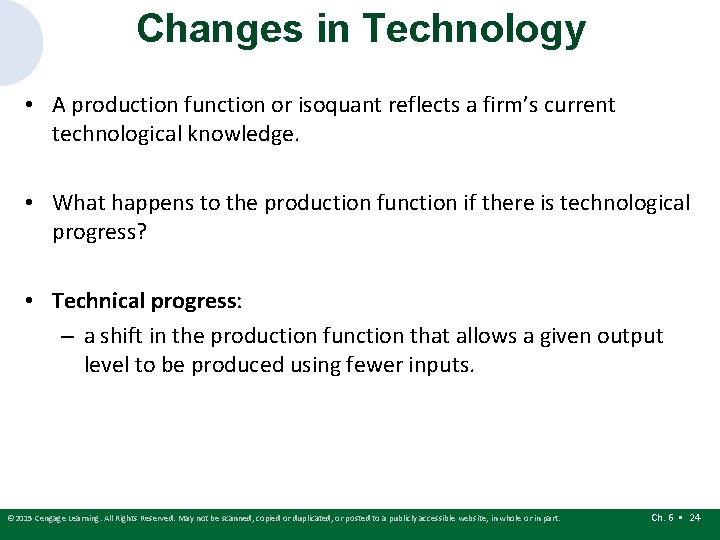
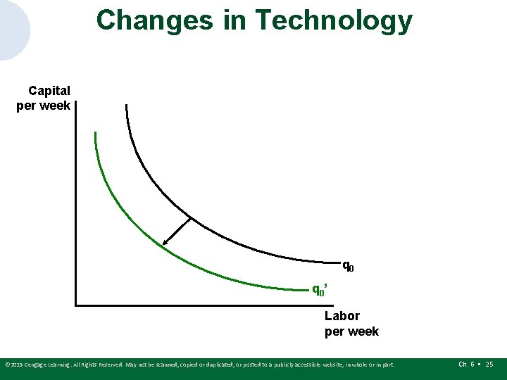
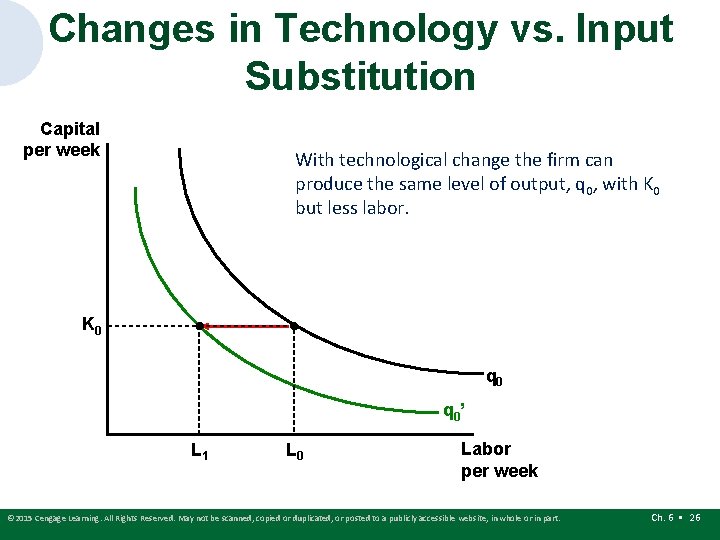
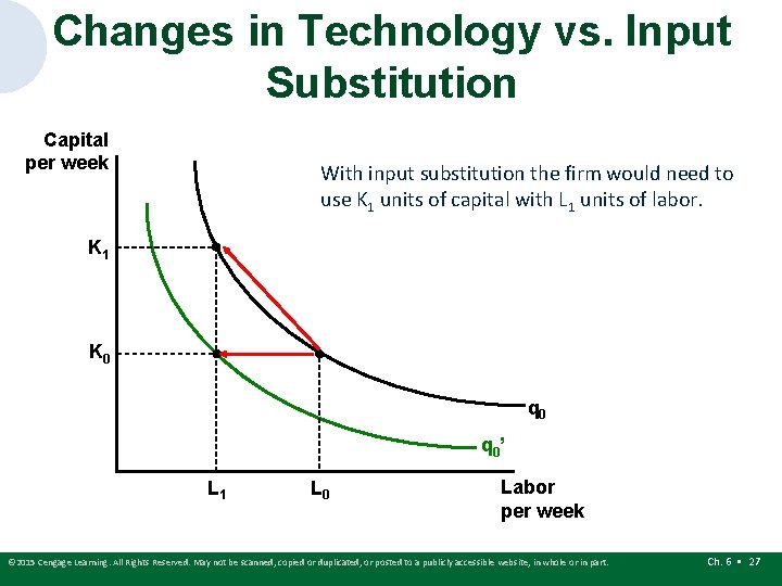
Changes in Technology • A production function or isoquant reflects a firm’s current technological knowledge. • What happens to the production function if there is technological progress? • Technical progress: – a shift in the production function that allows a given output level to be produced using fewer inputs. © 2015 Cengage Learning. All Rights Reserved. May not be scanned, copied or duplicated, or posted to a publicly accessible website, in whole or in part. Ch. 6 • 24

Changes in Technology Capital per week q 0 ’ Labor per week © 2015 Cengage Learning. All Rights Reserved. May not be scanned, copied or duplicated, or posted to a publicly accessible website, in whole or in part. Ch. 6 • 25

Changes in Technology vs. Input Substitution Capital per week With technological change the firm can produce the same level of output, q 0, with K 0 but less labor. K 0 q 0 ’ L 1 L 0 Labor per week © 2015 Cengage Learning. All Rights Reserved. May not be scanned, copied or duplicated, or posted to a publicly accessible website, in whole or in part. Ch. 6 • 26

Changes in Technology vs. Input Substitution Capital per week With input substitution the firm would need to use K 1 units of capital with L 1 units of labor. K 1 K 0 q 0 ’ L 1 L 0 Labor per week © 2015 Cengage Learning. All Rights Reserved. May not be scanned, copied or duplicated, or posted to a publicly accessible website, in whole or in part. Ch. 6 • 27

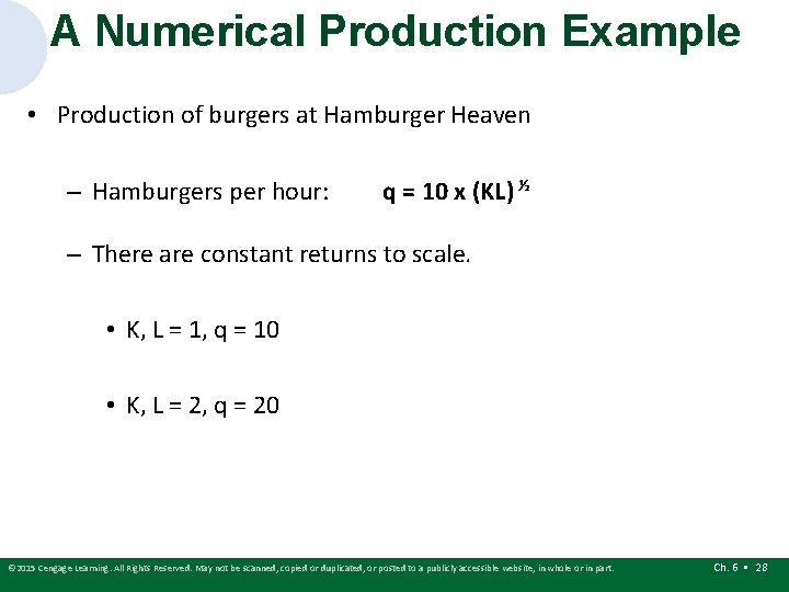
A Numerical Production Example • Production of burgers at Hamburger Heaven – Hamburgers per hour: q = 10 x (KL) ½ – There are constant returns to scale. • K, L = 1, q = 10 • K, L = 2, q = 20 © 2015 Cengage Learning. All Rights Reserved. May not be scanned, copied or duplicated, or posted to a publicly accessible website, in whole or in part. Ch. 6 • 28

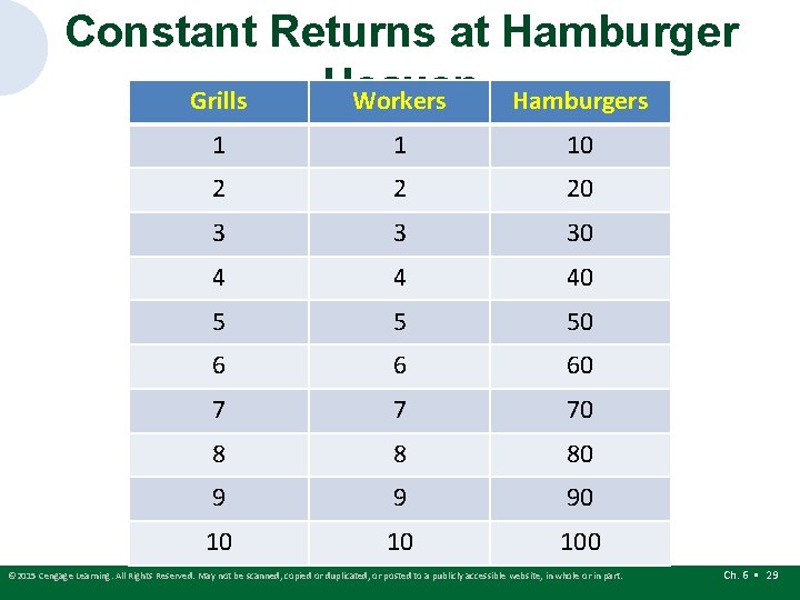
Constant Returns at Hamburger Heaven Grills Workers Hamburgers 1 1 10 2 2 20 3 3 30 4 4 40 5 5 50 6 6 60 7 7 70 8 8 80 9 9 90 10 10 100 © 2015 Cengage Learning. All Rights Reserved. May not be scanned, copied or duplicated, or posted to a publicly accessible website, in whole or in part. Ch. 6 • 29

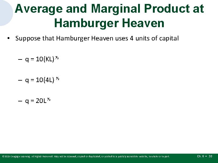
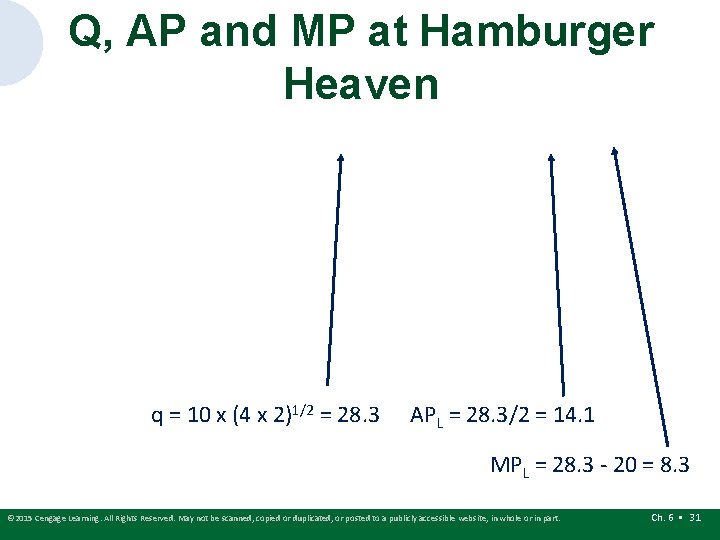
Average and Marginal Product at Hamburger Heaven • Suppose that Hamburger Heaven uses 4 units of capital – q = 10(KL) ½ – q = 10(4 L) ½ – q = 20 L ½ © 2015 Cengage Learning. All Rights Reserved. May not be scanned, copied or duplicated, or posted to a publicly accessible website, in whole or in part. Ch. 6 • 30

Q, AP and MP at Hamburger Heaven q = 10 x (4 x 2)1/2 = 28. 3 APL = 28. 3/2 = 14. 1 MPL = 28. 3 - 20 = 8. 3 © 2015 Cengage Learning. All Rights Reserved. May not be scanned, copied or duplicated, or posted to a publicly accessible website, in whole or in part. Ch. 6 • 31

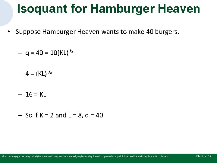
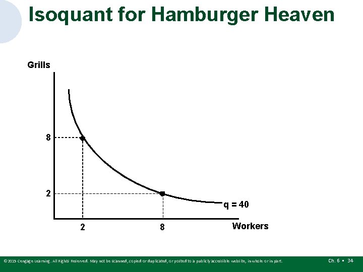
Isoquant for Hamburger Heaven • Suppose Hamburger Heaven wants to make 40 burgers. – q = 40 = 10(KL) ½ – 4 = (KL) ½ – 16 = KL – So if K = 2 and L = 8, q = 40 © 2015 Cengage Learning. All Rights Reserved. May not be scanned, copied or duplicated, or posted to a publicly accessible website, in whole or in part. Ch. 6 • 32

Isoquant for Hamburger Heaven © 2015 Cengage Learning. All Rights Reserved. May not be scanned, copied or duplicated, or posted to a publicly accessible website, in whole or in part. Ch. 6 • 33

Isoquant for Hamburger Heaven Grills 8 2 q = 40 2 8 Workers © 2015 Cengage Learning. All Rights Reserved. May not be scanned, copied or duplicated, or posted to a publicly accessible website, in whole or in part. Ch. 6 • 34

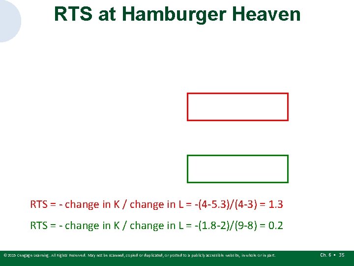
RTS at Hamburger Heaven RTS = - change in K / change in L = -(4 -5. 3)/(4 -3) = 1. 3 RTS = - change in K / change in L = -(1. 8 -2)/(9 -8) = 0. 2 © 2015 Cengage Learning. All Rights Reserved. May not be scanned, copied or duplicated, or posted to a publicly accessible website, in whole or in part. Ch. 6 • 35

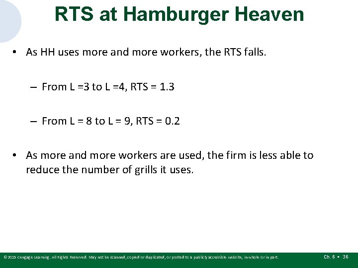
RTS at Hamburger Heaven • As HH uses more and more workers, the RTS falls. – From L =3 to L =4, RTS = 1. 3 – From L = 8 to L = 9, RTS = 0. 2 • As more and more workers are used, the firm is less able to reduce the number of grills it uses. © 2015 Cengage Learning. All Rights Reserved. May not be scanned, copied or duplicated, or posted to a publicly accessible website, in whole or in part. Ch. 6 • 36

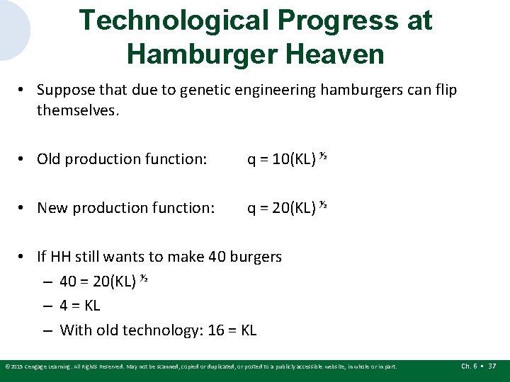
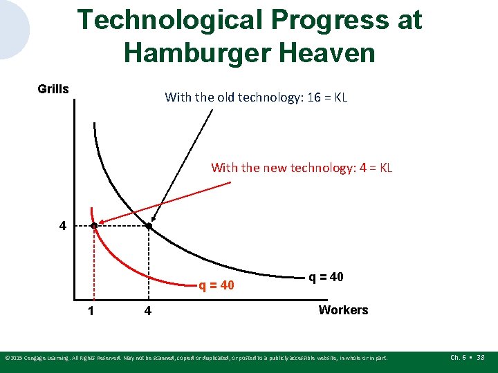
Technological Progress at Hamburger Heaven • Suppose that due to genetic engineering hamburgers can flip themselves. • Old production function: q = 10(KL) ½ • New production function: q = 20(KL) ½ • If HH still wants to make 40 burgers – 40 = 20(KL) ½ – 4 = KL – With old technology: 16 = KL © 2015 Cengage Learning. All Rights Reserved. May not be scanned, copied or duplicated, or posted to a publicly accessible website, in whole or in part. Ch. 6 • 37

Technological Progress at Hamburger Heaven Grills With the old technology: 16 = KL With the new technology: 4 = KL 4 q = 40 1 4 q = 40 Workers © 2015 Cengage Learning. All Rights Reserved. May not be scanned, copied or duplicated, or posted to a publicly accessible website, in whole or in part. Ch. 6 • 38

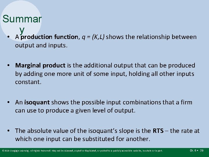
Summar y • A production function, q = (K, L) shows the relationship between output and inputs. • Marginal product is the additional output that can be produced by adding one more unit of some input, holding all other inputs constant. • An isoquant shows the possible input combinations that a firm can use to produce a given level of output. • The absolute value of the isoquant’s slope is the RTS – the rate at which one input can be substituted for another. © 2015 Cengage Learning. All Rights Reserved. May not be scanned, copied or duplicated, or posted to a publicly accessible website, in whole or in part. Ch. 6 • 39

Summar y • The RTS falls as the firm uses more and more of one input. • Production may exhibit constant, decreasing, or increasing returns to scale. • With fixed proportions production a firm will not be able to substitute one input for another. • With technological progress a firm can produce a given level of output with fewer inputs: the isoquant shifts in. © 2015 Cengage Learning. All Rights Reserved. May not be scanned, copied or duplicated, or posted to a publicly accessible website, in whole or in part. Ch. 6 • 40