Monitoraggio Geodetico e Telerilevamento 4 Image Classification Techniques

Monitoraggio Geodetico e Telerilevamento 4 Image Classification Techniques 1 Carla Braitenberg Dip. Matematica e Geoscienze Universita’ di Trieste berg@units. it

Image Classification (Chapter 7. 7 - of Lillesand et al. 2015) • Objective of Classification: replace visual interpretation with quantitative technqiues for automation of identification of features on the scene. • Determine statistical decision rules for determining the land cover of each pixel. • Spectral pattern recognition: classification based on spectral radiances • Spatial pattern recognition: decision rules based on geometric shapes, sizes and patterns of the data. • Hybrid methods: both spatial and spectral methods used for classification • Result is thematic map of land cover and summary statistics on the areas.

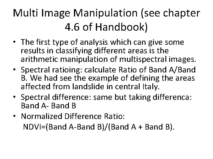
Multi Image Manipulation (see chapter 4. 6 of Handbook) • The first type of analysis which can give some results in classifying different areas is the arithmetic manipulation of multispectral images. • Spectral ratioing: calculate Ratio of Band A/Band B. We had see the example of defining the areas affected from landslide in central Italy. • Spectral difference: same but taking differenca: Band A- Band B • Normalized Difference Ratio: NDVI=(Band A-Band B)/(Band A + Band B).

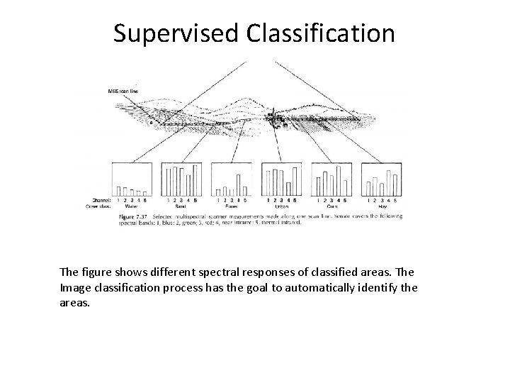
Supervised Classification The figure shows different spectral responses of classified areas. The Image classification process has the goal to automatically identify the areas.

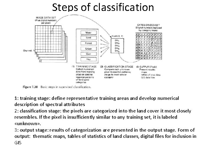
Steps of classification 1: training stage: define representative training areas and develop numerical description of spectral attributes 2: classification stage: the pixels are categorized into the land cover it most closely resembles. If the pixel is insufficiently similar to any training set, it is labeled «unknown» . 3: output stage: results of categorization are presented in the output stage. Form of output: thematic maps, tables of statistics of land classes, digital files for inclusion in GIS

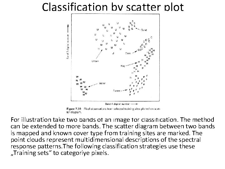
Classification by scatter plot For illustration take two bands of an image for classification. The method can be extended to more bands. The scatter diagram between two bands is mapped and known cover type from training sites are marked. The point clouds represent multidimensional descriptions of the spectral response patterns. The following classification strategies use these „Training sets“ to categoriye pixels.

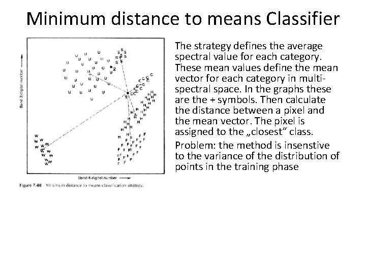
Minimum distance to means Classifier The strategy defines the average spectral value for each category. These mean values define the mean vector for each category in multispectral space. In the graphs these are the + symbols. Then calculate the distance between a pixel and the mean vector. The pixel is assigned to the „closest“ class. Problem: the method is insenstive to the variance of the distribution of points in the training phase

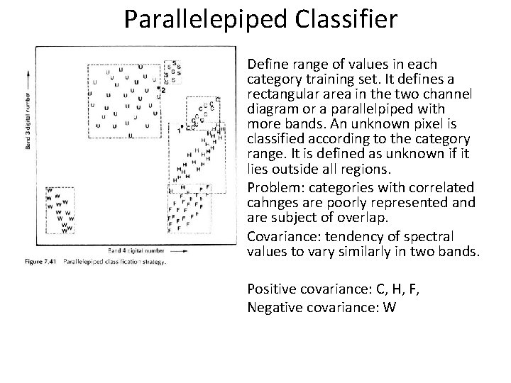
Parallelepiped Classifier Define range of values in each category training set. It defines a rectangular area in the two channel diagram or a parallelpiped with more bands. An unknown pixel is classified according to the category range. It is defined as unknown if it lies outside all regions. Problem: categories with correlated cahnges are poorly represented and are subject of overlap. Covariance: tendency of spectral values to vary similarly in two bands. Positive covariance: C, H, F, Negative covariance: W

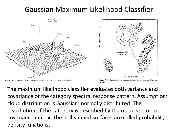
Gaussian Maximum Likelihood Classifier The maximum likelihood classifier evaluates both variance and covariance of the category spectral response pattern. Assumption: cloud distribution is Gaussian=normally distributed. The distribution of the category is described by the mean vector and covariance matrix. The bell-shaped surfaces are called probability density functions.

Gaussian Maximum Likelihood Classifier cont. • The probability density functions are used to classify a pixel by computing the probability of the pixel value belonging to each category. The pixel is assigned to the most likely class, equal to the highest probability value. • The maximum likelyhood classifier delineates ellipsoidal equiprobablity contours in the scatter diagram. • An extension is the Bayesian classifier: two weighting factors are applied to the probability estimate. First the analyst gives the «a priori probability» . This is the anticipated likelihood of occurrence of each class in the scene. Second, a weight associated with the cost of mis-classification applied to each class. Together, these factors act to minimize the cost of misclassification, resulting in an optimum classification. • In practice, most maximum likelihood classification is done assuming equal probability of occurrence and cost of misclassification for all classes.

Training Stage • Classification of multispectral images is automatic - assembling and training data needed for classification requires attention by the analyst. • Objective of training process: assemble set of statistics that describe spectral response pattern of each land cover type to be classified. In the training stage the clods of points are determined. Training data must be representative and complete. One information class may be represented by different spectral classes. Example: to delineate the information class water, the spectral properties could depend on having clear water, turbid water, requiring at least two spectral classes.

Training class agriculture • Might contain several spectral classes. Could stem from: planting dates, soil moisture conditions, crop management practices, seed varieties, topographic setting, atmospheric conditions • An image can requires up to 100 or more training areas to adequately represent the spectral variability.