Monitoraggio Geodetico e Telerilevamento Earth Engine exercizes Carla

Monitoraggio Geodetico e Telerilevamento Earth. Engine exercizes Carla Braitenberg Dip. Matematica e Geoscienze Universita’ di Trieste berg@units. it Tel. 339 8290713 Tel. Assistente Dr. Nagy: 040 5582257

Please follow the next scripts • https: //code. earthengine. google. com/ • Javascript Reference: https: //www. w 3 schools. com/js/js_math. asp

Script 00 introduction to scripter language • • • // String objects can also start and end with double quotes. // But don't mix and match them. var my_other_variable = "I am also a string"; • • // Statements should end in a semi-colon, or the editor complains. var test = 'I feel incomplete. . . ' • • // Parentheses are used to pass parameters to functions. print('This string will print in the Console tab. '); • • • // Square brackets are used for selecting items within a list. // The zero index refers to the first item in the list. var my_list = ['eggplant', 'apple', 'wheat']; print(my_list[0]); var the_answer=42; // Curly brackets (or braces) can be used to define dictionaries (key: value pairs) var my_dict = {'food': 'bread', 'color': 'red', 'number': the_answer}; // Square brackets can be used to access dictionary items by key. print(my_dict['number']); print(my_dict['color']); // Or you can use the dot notation to get the same result. print(my_dict. color); • • • // Functions can be defined as a way to reuse code and make it easier to read var my_hello_function = function(string) { return 'Hello ' + string + '!'; }; print(my_hello_function('world')); Further comments to this introduction: https: //developers. google. com/ earth-engine/tutorial_js_01

Script 00 -Continues introduction to scripter language • • • // define sum and multiplication in function var my_sum_function = function(s 1, s 2) { var t 3=[s 1+s 2, s 1*s 2] return t 3; }; print(my_sum_function(2, 3)); Access other possible numerical operations: Create object of type number in ee: var s 1=1. 3 var t 5 = ee. Number(s 1) Call the method cos which you find in the documentation Docs for the object ee. Number: var t 6 = t 5. cos() Equivalent: Var t 6=ee. Number(s 1). cos() Equivalent- basic Javascript instructions (see Javascript guide): Var t 6=Math. cos(s 1)

01 Script var srtm = ee. Image("USGS/SRTMGL 1_003"); Map. add. Layer(srtm, {min: 0, max: 3000}); // Get a list of all metadata properties. var properties = srtm. property. Names(); print('Metadata properties: ', properties); // ee. List of metadata properties // Get a specific metadata property. var d = srtm. get('date_range'); print('daterange: ', d); var p = srtm. get('title'); print('title: ', p);

• • • • • • • 02 script // Using mathematical functions // Functions can be defined as a way to reuse code and make it easier to read var my_hello_function = function(string) { return 'Hello ' + string + '!'; }; print(my_hello_function('world')); // define sum and multiplication in function var my_sum_function = function(s 1, s 2) { var t 3=[s 1+s 2, s 1*s 2] return t 3 }; print(my_sum_function (4, 5)) // define sum and multiplication in function var my_sum_function = function(s 1, s 2) { var t 4= s 1+s 2 var t 3 =s 1*s 2 var t 5 = ee. Number(s 1) var t 6 = t 5. cos() return [t 3, t 4, t 6]; }; var tg = my_sum_function(2, 3); print(tg) // useful sometimes: get present date: var d = new Date(); print(d)

Script 03 • var srtm = ee. Image("USGS/SRTMGL 1_003"); var slope = ee. Terrain. slope(srtm); • Map. add. Layer(srtm, {min: 0, max: 3000}, 'DEM'); • Map. add. Layer(slope, {min: 0, max: 10}, 'slope'); ee. Terrain. slope(): Calculates slope in degrees from a terrain DEM. The local gradient is computed using the 4 -connected neighbors of each pixel, so missing values will occur around the edges of an image. Arguments: input (Image): An elevation image, in meters. Returns: Image

Script 03 continues • var srtm = ee. Image("USGS/SRTMGL 1_003"); • • • // we compute the slope explicitly // Compute the image gradient in the X and Y directions. var xy. Grad = srtm. gradient(); • • • • • // Compute the magnitude of the gradient. var gradient =( xy. Grad. select('x'). pow(2) . add(xy. Grad. select('y'). pow(2))). sqrt(); // Compute slope angle in radians var slope 1 = gradient. atan(); // Compute the slope angle in degrees using an expression. var slopedeg = slope 1. expression( '180*1. 0/3. 1415926535*sl', { 'sl': slope 1 }); // Compute the direction of the gradient in radians var direction = xy. Grad. select('y'). atan 2(xy. Grad. select('x')); // Display the results. Map. set. Center(12, 45, 10); Map. add. Layer(direction, {min: -2, max: 2, format: 'png'}, 'direction'); Map. add. Layer(gradient, {min: -0. 01, max: 0. 02, format: 'png'}, 'gradient'); Map. add. Layer(slopedeg, {min: 0, max: 10, format: 'png'}, 'slope 1');

Script 04 • var landsat 8 = ee. Image. Collection("LANDSAT/LC 8_L 1 T_TOA"); • var images = landsat 8. filter. Date('2015 -04 -01', '2015 -04 -06'); • Map. add. Layer(images); Dettagli sulla missione Landsat Vedi documentazione della NASA https: //landsat. gsfc. nasa. gov/landsat-data-continuity-mission/ Esempi di immagini a diverse bande di frequenza: https: //landsat. gsfc. nasa. gov/landsat-8 -bands/

Landsat 8 - summary • • Landsat 8 launched on February 11, 2013, from Vandenberg Air Force Base, California, on an Atlas-V 401 rocket, with the extended payload fairing
 (EPF) from United Launch Alliance, LLC. The Landsat 8 satellite payload consists of two science instruments—the Operational Land Imager (OLI) and the Thermal Infrared Sensor (TIRS). These two sensors provide seasonal coverage of the global landmass at a spatial resolution of 30 meters (visible, NIR, SWIR); 100 meters (thermal); and 15 meters (panchromatic). Landsat 8 instruments represent an evolutionary advance in technology. OLI improves on past Landsat sensors. OLI is a push-broom sensor with a four-mirror telescope and 12 -bit quantization. OLI collects data for visible, near infrared, and short wave infrared spectral bands as well as a panchromatic band. It has a fiveyear design life. The graphic below compares the OLI spectral bands to Landsat 7′s ETM+ bands. OLI provides two new spectral bands, the coastal band (band 1) and a cirrus cloud band (band 9),

Comparison of spectral bands of Landsat 8 and Landsat 7

Landsat 1 Launch Date: July 23, 1972 Status: expired, January 6, 1978 Sensors: RBV, MSS Altitude: nominally 900 km Inclination: 99. 2° Orbit: polar, sun-synchronous Equatorial Crossing Time: nominally 9: 42 AM mean local time (descending node) • Period of Revolution : 103 minutes; ~14 orbits/day • Repeat Coverage : 18 days • •

Script 04 • var landsat 8 = ee. Image. Collection("LANDSAT/LC 8_L 1 T_TOA"); • var images = landsat 8. filter. Date('2015 -04 -01', '2015 -04 -06'); • Map. add. Layer(images); Per esercizio: variare i periodi temporali Consultare le proprieta’ del database Landsat 8. Caricare un altro database, per esempio sentinel 2 o landsat 7. Confrontare con le proprieta’ di landsat 7. Attenzione a scegliere le date opportune avendo controllato la copertura sulla documentazione. Begin 2 may 2018.

Script 04 -continua var landsat 8 = ee. Image. Collection("LANDSAT/LC 8_L 1 T_TOA"); var images = landsat 8. filter. Date('2015 -04 -01', '2015 -04 -06'); Map. add. Layer(images); Ispezionare le proprieta’ della figura in scala di grigi nel menu “Inspector” Nell’imagine sono sovrapposte tutte le bande facenti parte della collezione. Nel prossimo script selezioniamo le bande del visibile e dell’infrarosso.

Script 05 var landsat 8 = ee. Image. Collection("LANDSAT/LC 8_L 1 T_TOA"); var rgb_viz = {min: 0, max: 0. 3, bands: ['R', 'G', 'B']}; var rgb_viz 1 = {min: 0, max: 0. 3, bands: ['B', 'G', 'R']}; var images = landsat 8. select(['B 2', 'B 3', 'B 4', 'B 5'], ['B', 'G', 'R', 'N']); images = images. filter. Date('2015 -04 -01', '2015 -04 -06'); Map. add. Layer(images, rgb_viz, 'True Color'); Map. add. Layer(images, rgb_viz 1, 'False Color');

Script 6 Median var landsat 8 = ee. Image. Collection("LANDSAT/LC 8_L 1 T_TOA"); var rgb_viz = {min: 0, max: 0. 3, bands: ['R', 'G', 'B']}; var images = landsat 8. select(['B 2', 'B 3', 'B 4', 'B 5'], ['B', 'G', 'R', 'N']); images = images. filter. Date('2015 -04 -01', '2015 -10 -06'); Map. add. Layer(images, rgb_viz, 'True Color'); Map. add. Layer(images. median(), rgb_viz, 'True Color median'); Next to median, you have also: mode and mean. Median: Middle value separating the greater and lesser halves of a data set Mode: Most frequent value in a data set Mean: Sum of values of a data set divided by number of values

Script 7 Sentinel var sentinel 2 = ee. Image. Collection("COPERNICUS/S 2"); var landsat 8 = ee. Image. Collection("LANDSAT/LC 8_L 1 T_TOA"); var rgb_viz = {min: 0, max: 0. 3, bands: ['R', 'G', 'B']}; var rgb_viz 2 = {min: 0, max: 2000, bands: ['R', 'G', 'B']}; var images = landsat 8. select(['B 2', 'B 3', 'B 4', 'B 5'], ['B', 'G', 'R', 'N']); var images 2 = sentinel 2. select(['B 2', 'B 3', 'B 4', 'B 5'], ['B', 'G', 'R', 'N']); images = images. filter. Date('2016 -05 -01', '2016 -05 -06'); images 2 = images 2. filter. Date('2016 -01 -26', '2016 -04 -28'); Map. add. Layer(images, rgb_viz, 'True Color'); Map. add. Layer(images 2, rgb_viz 2, 'True Color sentinel'); Map. add. Layer(images. median(), rgb_viz, 'True Color median');

Script 7 Sentinel- filter on location var landsat 8 = ee. Image. Collection("LANDSAT/LC 8_L 1 T_TOA"); var s 2 = ee. Image. Collection("COPERNICUS/S 2"); var geometry = /* color: 0000 ff */ee. Geometry. Point([13, 45. 5]); // // Landsat 8 // var images = landsat 8. select(['B 2', 'B 3', 'B 4', 'B 5'], ['B', 'G', 'R', 'N']); // var rgb_viz = {min: 0, max: 0. 3, bands: ['R', 'G', 'B']}; // Sentinel 2 var images = s 2. select(['B 2', 'B 3', 'B 4', 'B 8'], ['B', 'G', 'R', 'N']); var rgb_viz = {min: 0, max: 2000, bands: ['R', 'G', 'B']}; images = images. filter. Date('2015 -08 -01', '2015 -12 -11'); images = images. filter. Bounds(geometry); var sample = ee. Image(images. first()); Map. add. Layer(sample, rgb_viz, 'sample'); Map. add. Layer(images. median(), rgb_viz, 'True Color median');

Script 8 sentinel Min-max • • var s 2 toa = ee. Image. Collection("COPERNICUS/S 2"); var rgb_viz = {min: 0, max: 2000, bands: ['R', 'G', 'B']}; var s 2 = s 2 toa. select(['B 2', 'B 3', 'B 4', 'B 5'], ['B', 'G', 'R', 'N']) . filter. Date('2016 -01 -26', '2016 -04 -28'); print(s 2. size()); Map. add. Layer(s 2, rgb_viz, 'RGB'); Map. add. Layer(s 2. max(), rgb_viz, 'max'); Map. add. Layer(s 2. min(), rgb_viz, 'min');

Script 9 NDVI var s 2 toa = ee. Image. Collection("COPERNICUS/S 2"); var rgb_viz = {min: 0, max: 2000, bands: ['R', 'G', 'B']}; var s 2 = s 2 toa. select(['B 2', 'B 3', 'B 4', 'B 5'], ['B', 'G', 'R', 'N']) . filter. Date('2016 -01 -26', '2016 -04 -28'); print(s 2. size()); Map. add. Layer(s 2, rgb_viz, 'RGB', false); var image = s 2. min(); Map. add. Layer(image, rgb_viz, 'image'); var ndvi = image. normalized. Difference(['N', 'R']); var ndwi_viz = {min: -0. 2, max: 0. 2, palette: 'black, green'}; • Map. add. Layer(ndvi, ndwi_viz, 'NDVI'); • • • NDVI=(NIR-Red)/(NIR+Red) Normalized Difference vegetation Index end 3 may 2018.

Script 10 sediment identification Example from Caribbean Sea. The problem is to identify the sediment input from the River and detect the seasonal changes of the size and form of the sediment cloud. This is done from multispectral Landsat images. var landsat 8 = ee. Image. Collection("LANDSAT/LC 08/C 01/T 1_SR"); var landsat 7 = ee. Image. Collection("LANDSAT/LE 07/C 01/T 1_SR"); //var landsat 8 = ee. Image. Collection("LANDSAT/LC 8_L 1 T_TOA"), // landsat 7 = ee. Image. Collection("LANDSAT/LE 7_L 1 T_TOA"); var rgb_viz = {min: 0, max: 1500, bands: ['R', 'G', 'B']}; var rgb_viz 1 = {min: 0, max: 1500, bands: ['B', 'G', 'N']}; var images = landsat 8. select(['B 2', 'B 3', 'B 5', 'B 4'], ['B', 'G', 'N', 'R']); var images 7 = landsat 7. select(['B 1', 'B 2', 'B 4', 'B 3'], ['B', 'G', 'N', 'R']); var geometry = /* color: 0000 ff */ee. Geometry. Point([-75, 11]); images = images. filter. Date('2015 -04 -01', '2015 -04 -06'); images = images. filter. Bounds(geometry); images 7 = images 7. filter. Date('2000 -04 -01', '2000 -12 -30'); images 7 = images 7. filter. Bounds(geometry); Map. add. Layer(images, rgb_viz, 'True Color L 8'); Map. add. Layer(images, rgb_viz 1, 'False Color L 8'); Map. add. Layer(images 7, rgb_viz, 'True Color L 7'); Map. add. Layer(images 7, rgb_viz 1, 'False Color L 7'); Begin 9 may 2018.

False color image compared to true image Landsat 8 (april 2015

Landsat 7 April 2000

sediment identification by histogram analysis The histograms were generated in Earth Engine for the Caribbean Sea. The near infrared level is similar, the B, G, R levels are higher where sediments are suspended in water. B G N R Water with sediments Water without sediments

Distinction of water covered areas from land areas • Modifying the bands used for the false images we can distinguish water covered areas better from land areas. • This can be accomplished by using the bands N and either one of B, G, R.

Calculate the difference between the two dates • Operations: select Landsat 7 and landsat 8 as in previous excersize, apply a reducer to obtain two single images, then calculate the difference between the two images. At last map the difference image, taking care of the much smaller values, so you must adjust the color-scale accordingly.

var landsat 8 = ee. Image. Collection("LANDSAT/LC 08/C 01/T 1_SR"); var landsat 7 = ee. Image. Collection("LANDSAT/LE 07/C 01/T 1_SR"); //var landsat 8 = ee. Image. Collection("LANDSAT/LC 8_L 1 T_TOA"); //landsat 7 = ee. Image. Collection("LANDSAT/LE 7_L 1 T_TOA"); var rgb_viz = {min: 0, max: 1500, bands: ['R', 'G', 'B']}; var rgb_viz 1 = {min: 0, max: 1500, bands: ['B', 'G', 'N']}; var images = landsat 8. select(['B 2', 'B 3', 'B 5', 'B 4'], ['B', 'G', 'N', 'R']); var images 7 = landsat 7. select(['B 1', 'B 2', 'B 4', 'B 3'], ['B', 'G', 'N', 'R']); var geometry = /* color: 0000 ff */ee. Geometry. Point([-75, 11]); images = images. filter. Date('2015 -04 -01', '2015 -04 -06'); images = images. filter. Bounds(geometry); images 7 = images 7. filter. Date('2000 -04 -01', '2000 -12 -30'); images 7 = images 7. filter. Bounds(geometry); var imagesmin = images. min(); var images 7 min = images 7. min(); // calculate normalized difference index between blue and near infrared. Image collection must be reduced before. var ndvi = imagesmin. normalized. Difference(['B', 'N']); var ndwi_viz = {min: -0. 4, max: 0. 4, palette: 'black, green'}; // calculate difference between situation in 2015 and 2000. You must reduce image collection before. var diff = imagesmin. subtract(images 7 min); Map. set. Center(-75, 11, 10); Map. add. Layer(diff, {bands: ['B', 'G', 'N'], min: -500, max: 500}, 'difference'); Map. add. Layer(ndvi, ndwi_viz, 'ndvi'); Map. add. Layer(images, rgb_viz, 'True Color L 8', 'false'); Map. add. Layer(images, rgb_viz 1, 'False Color L 8', 'false');

Difference in false colors. Purple area in oceanic marks the change in suspendedsediment density

Script 11 Distinguish water from land covered areas var landsat 8 = ee. Image. Collection("LANDSAT/LC 8_L 1 T_TOA"); var rgb_viz = {min: 0, max: 0. 3, bands: ['R', 'G', 'B']}; var rgb_viz 1 = {min: 0, max: 0. 3, bands: ['B 5', 'B 6', 'B 7']}; var images = landsat 8. select(['B 2', 'B 3', 'B 5', 'B 4'], ['B', 'G', 'N', 'R']); var images_water = landsat 8. select(['B 5', 'B 6', 'B 7']); var geometry = ee. Geometry. Multi. Point([12, 45, 14, 46]); images = images. filter. Date('2015 -04 -01', '2015 -04 -30'); images = images. filter. Bounds(geometry); images_water = images_water. filter. Date('2015 -04 -01', '2015 -04 -30'); images_water = images_water. filter. Bounds(geometry); Map. add. Layer(images, rgb_viz, 'True Color L 8'); Map. add. Layer(images_water. min(), rgb_viz 1, 'False Color L 8');

Laguna Grado- false colors Landsat 8

Script 12 Birth of an Island • Between September and October 2013 in the Red Sea an Island was born. This can be well seen in the Landsat 8 images. To enhance the signal we display both the true color and the false color image before and after the appearance of the island. The approximate coordinate of the area of interest is the following: Long 42. 1367, 15. 0960 • Reference: http: //www. nature. com/ncomms/2015/150526/ncomms 8104/pdf/ncomms 8104. pdf • • • Possible other island birth to be observed: april 2015, between two Tonga islands Reference: Garvin, J. B. , Slayback, D. A. , Ferrini, V. , Frawley, J. , Giguere, C. , Asrar, G. R. , & Andersen, K. (2018). Monitoring and modeling the rapid evolution of Earth’s newest volcanic island: Hunga Tonga Hunga Ha’apai (Tonga) using high spatial resolution satellite observations. Geophysical Research Letters, 45. https: //doi. org/10. 1002/2017 GL 076621 DOI: 10. 1002/2017 GL 076621 • •

• • var landsat 8 = ee. Image. Collection("LANDSAT/LC 8_L 1 T_TOA"), geometry = /* color: ffc 82 d */ee. Geometry. Point([42. 136688232421875, 15. 095991084505304]); var rgb_viz = {min: 0, max: 0. 3, bands: ['R', 'G', 'B']}; var rgb_viz 1 = {min: 0, max: 0. 3, bands: ['B 5', 'B 6', 'B 7']}; • • var images = landsat 8. select(['B 2', 'B 3', 'B 5', 'B 4'], ['B', 'G', 'N', 'R']); var images 1 = landsat 8. select(['B 2', 'B 3', 'B 5', 'B 4'], ['B', 'G', 'N', 'R']); var images_water = landsat 8. select(['B 5', 'B 6', 'B 7']); var images_water 1 = landsat 8. select(['B 5', 'B 6', 'B 7']); • • • • var geometry = ee. Geometry. Point([42, 15]); images 1 = images 1. filter. Date('2013 -04 -01', '2013 -07 -01'); images 1 = images 1. filter. Bounds(geometry); images = images. filter. Date('2013 -11 -1', '2013 -12 -30'); images = images. filter. Bounds(geometry); images_water 1 = images_water 1. filter. Date('2013 -08 -01', '2013 -09 -11'); images_water 1 = images_water 1. filter. Bounds(geometry); images_water = images_water. filter. Date('2013 -11 -1', '2013 -12 -30'); images_water = images_water. filter. Bounds(geometry); Map. set. Center(42, 15, 10); Map. add. Layer(images 1. min(), rgb_viz, 'before'); Map. add. Layer(images. min(), rgb_viz, 'after'); Map. add. Layer(images_water 1, rgb_viz 1, 'False Color before'); Map. add. Layer(images_water, rgb_viz 1, 'False Color after'); •

Island birth in Red Sea BEFORE AFTER images 1. filter. Date('2013 -04 -01', '2013 -07 -01'); images. filter. Date('2013 -11 -1', '2013 -12 -30'); Landsat 8. Bands 'B 5', 'B 6', 'B 7

Script 13 - Cycle through Landsat Images over the same spot • Scope is to select landsat images through time on the same spot, using the first image of successive Landsat missions

Script 13 - Cycle through Landsat Images over the same spot • // Compare MSS images from L 1 through L 5 • var sf. Point = ee. Geometry. Point(31. 267, 30. 031); • Map. set. Center(31. 267, 30. 031, 10); //var sf. Point = ee. Geometry. Point(13. , 45. 3); this for images centered close to Trieste //Map. set. Center(13, 45. 3, 10); • • • for (var i = 1; i <= 5; ++i) { var collection = ee. Image. Collection('LM' + i + '_L 1 T'); var image = ee. Image(collection. filter. Bounds(sf. Point). first()); var toa = ee. Algorithms. Landsat. TOA(image); var date = ee. Date(image. get('system: time_start')). format('MMM yyyy'); var bands = (i <= 3) ? ['B 6', 'B 5', 'B 4'] : ['B 2', 'B 3', 'B 1']; // This is one of the rare places where we need to use get. Info() in the // middle of a script, since layer names must be client-side strings. var label = 'Landsat' + i + ' (' + date. get. Info() + ')'; Map. add. Layer(toa, {bands: bands, min: 0, max: 0. 4}, label); }

• • • • • • Script 13 b- as before with display time variation on chart // Compare MSS images from L 1 through L 5 var sf. Point = ee. Geometry. Point(31. 314, 30. 2); Map. set. Center(31. 314, 30. 2, 10); //var sf. Point = ee. Geometry. Point(13. , 45. 3); this for images centered close to Trieste //Map. set. Center(13, 45. 3, 10); for (var i = 1; i <= 5; ++i) { var collection = ee. Image. Collection('LM' + i + '_L 1 T'); var image = ee. Image(collection. filter. Bounds(sf. Point). first()); var toa = ee. Algorithms. Landsat. TOA(image); var date = ee. Date(image. get('system: time_start')). format('MMM yyyy'); var bands = (i <= 3) ? ['B 6', 'B 5', 'B 4'] : ['B 2', 'B 3', 'B 1']; // This is one of the rare places where we need to use get. Info() in the // middle of a script, since layer names must be client-side strings. var label = 'Landsat' + i + ' (' + date. get. Info() + ')'; Map. add. Layer(toa, {bands: bands, min: 0, max: 0. 4}, label); if (i <= 3) { print(Chart. image. series(collection. select('B 6'), sf. Point)); } else { print(Chart. image. series(collection. select('B 2'), sf. Point)); } }

Some explanations of script 13 for (var i = 1; i <= 5; ++i) { // this to repeat the following lines 5 times. var collection = ee. Image. Collection('LM' + i + '_L 1 T'); //this to change name of collection var image = ee. Image(collection. filter. Bounds(sf. Point). first()); var toa = ee. Algorithms. Landsat. TOA(image); // apply a correction to these crude images. TOA is top of Atmosphere var date = ee. Date(image. get('system: time_start')). format('MMM yyyy'); //find date of the selected image var bands = (i <= 3) ? ['B 6', 'B 5', 'B 4'] : ['B 2', 'B 3', 'B 1']; //for landsat 1 to 3, use bands B 6, B 5; B 4, else use B 3, B 2, B 1 (see next page for docu on landsat 1) // This is one of the rare places where we need to use get. Info() in the // middle of a script, since layer names must be client-side strings. var label = 'Landsat' + i + ' (' + date. get. Info() + ')'; //prepare the label including the date Map. add. Layer(toa, {bands: bands, min: 0, max: 0. 4}, label); }

Landsat 1 documentation • Multispectral Scanner (MSS) • 80 -meter ground resolution in four spectral bands: – Band 4 Visible green (0. 5 to 0. 6 µm) – Band 5 Visible red (0. 6 to 0. 7 µm) – Band 6 Near-Infrared (0. 7 to 0. 8 µm) – Band 7 Near-Infrared (0. 8 to 1. 1 µm) • Six detectors for each spectral band provided six scan lines on each active scan • Ground Sampling Interval (pixel size): 57 x 79 m

The bands of the MSS sensor on Landsat 1 -5 • https: //landsat. usgs. gov/what-are-band-designations-landsat-satellites

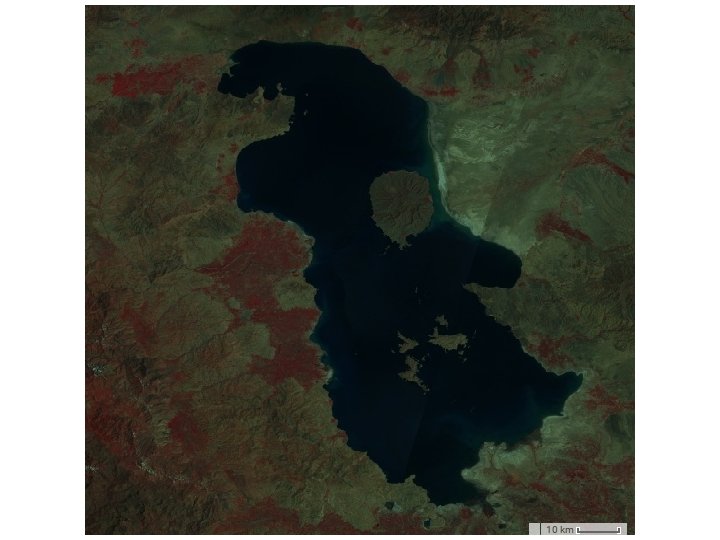
Corso di Monitoraggio Geodetico e Telerilevamento Esempio di schede powerpoint portate all’esame • Drying of Lake Urmia Di Felice Andrea

Lago Urmia • Il lago di Urmia e' un lago salato endoreico situato tra le province iraniane dell'Azerbaigian Orientale e dell'Azerbaigian Occidentale, a occidente del Mar Caspio. Fonte: Google Earth Engine È il maggiore dei laghi interni dell'Iran, con una superficie di circa 5. 200 km². Nel periodo di piena misura circa 140 km in lunghezza e 55 km in larghezza, ed ha una profondità massima di 16 m.

• • A causa del tasso di evaporazione elevato (da 600 mm a 1. 000 mm all'anno), il lago di Urmia è in continua fase di restringimento. Per tale motivo, il tasso di salinità del lago , lo rende inadatto alla vita di qualsiasi specie di pesce. Map. set. Center(45. 39, 37. 7099); Lago. Urmia nel 1985 Lago Urmia nel 2015 Fonte: Google Earth Engine Fonte: http: //eol. jsc. nasa. gov/sseop/EFS/photoinfo. pl? PHOTO=STS 41 G-37 -84

• • • Per lo studio dell'evoluzione del Lago Urmia si sono utilizzati rispettivamente i satelliti (esempio 14) -Landsat 4 (Periodo: Gennaio Giugno 1991). -Landsat 5 (Periodo : Gennaio-Giugno 2010 ). -Landsat 7 (Periodo: Gennaio-Giugno 2003). -Landsat 8 (Periodo : Gennaio-Giugno 2015). -Sentinel 2 (Periodo: Luglio 2016). • • var land 7 = ee. Image. Collection("LANDSAT/LE 7_L 1 T_TOA"), land 8 = ee. Image. Collection("LANDSAT/LC 8_L 1 T_TOA"), land 4 = ee. Image. Collection("LANDSAT/LT 4_L 1 T_TOA"), land 5 = ee. Image. Collection("LANDSAT/LT 5_L 1 T_TOA"), geometry 3 = /* color: #0 b 4 a 8 b */ee. Geometry. Multi. Point( [[45. 318603515625, 37. 65773212628272], [45. 120849609375, 38. 0740414594196], [45. 692138671875, 37. 142803443716865]]);

• • var rgb_viz = {min: 0, max: 0. 3, bands: ['R', 'G', 'B']}; var rgb_viz 1 = {min: 0, max: 0. 3, bands: ['B', 'G', 'R']}; • • • var land 8 = land 8. select(['B 4', 'B 3', 'B 2'], ['R', 'G', 'B']); //L 8 var land 8=land 8. filter. Bounds(geometry 3); var land 8= land 8. filter. Date('2015 -01 -05', '2015 -06 -30'); • • • var land 7 = land 7. select (['B 3', 'B 2', 'B 1'] , ['R', 'G', 'B']); var land 7=land 7. filter. Bounds(geometry 3); var land 7= land 7. filter. Date('2003 -01 -01' , '2003 -06 -30'); • • • var land 4 = land 4. select(['B 3', 'B 2', 'B 1', 'B 4'] , ['R', 'G', 'B', 'N']); var land 4=land 4. filter. Bounds(geometry 3); var land 4=land 4. filter. Date('1991 -01 -01', '1991 -06 -30'); • • • var land 5 = land 5. select(['B 3', 'B 2', 'B 1'], ['R', 'G', 'B']); var land 5 = land 5. filter. Date('2010 -01 -01', '2010 -06 -30'); var land 5 = land 5. filter. Bounds(geometry 3); • • • Map. add. Layer(land 4, rgb_viz, 'L 4 -91'); Map. add. Layer(land 7. median(), rgb_viz, 'L 7 -03', false); Map. add. Layer(land 5. median(), rgb_viz, 'L 5 -10', false); //Map. add. Layer(land 5. median(), rgb_viz 1, 'L 5 -10 FC', false); Map. add. Layer(land 8. median(), rgb_viz, 'L 8 -15', false); //Map. add. Layer(land 8. median(), rgb_viz 1, 'L 8 -15 FC', false); Le bande utilizzate per l'analisi sono state quelle corrispondenti ai 3 colori primari : Rosso , Verde , Blu. Le immagini sono state analizzate in colori reali(RGB).

• • • var s 2= ee. Image. Collection("COPERNICUS/S 2"); var rgb_vis = {min: 0, max: 2000, bands: ['R', 'G', 'B']}; var s 2= s 2. select(['B 2', 'B 3', 'B 4'], ['B', 'G', 'R']); var s 2=s 2. filter. Date('2016 -07 -01', '2016 -07 -30') var s 2=s 2. filter. Bounds(geometry 3); Map. add. Layer(s 2. median(), rgb_vis, 'S 2 -16 algaebloom. TC', false);

var land 5 = land 5. filter. Date('1985 -04 -01', '1985 -08 -30'); var land 5 = land 5. filter. Bounds(geometry); var land 4 = land 4. select(['B 3', 'B 2', 'B 1', 'B 4'] , ['R', 'G', 'B', 'N' var land 4=land 4. filter. Bounds(geometry 3); var land 4=land 4. filter. Date('1991 -01 -01', '1991 -06 -30');

var land 7 = land 7. select (['B 3', 'B 2', 'B 1'] , ['R', 'G', 'B']); var land 7=land 7. filter. Bounds(geometry 3); var land 7= land 7. filter. Date('2003 -01 -01' , '2003 -06 -30'); var land 5 = land 5. select(['B 3', 'B 2', 'B 1'], ['R', 'G', 'B']); var land 5 = land 5. filter. Date('2010 -01 -01', '2010 -06 -30'); var land 5 = land 5. filter. Bounds(geometry 3);

var land 8 = land 8. select(['B 4', 'B 3', 'B 2'], ['R', 'G', 'B']); //L 8 var land 8=land 8. filter. Bounds(geometry 3); var land 8= land 8. filter. Date('2015 -01 -05', '2015 -06 -30'); var s 2= s 2. select(['B 2', 'B 3', 'B 4'], ['B', 'G', 'R']); var s 2=s 2. filter. Date('2016 -07 -01', '2016 -07 -30') var s 2=s 2. filter. Bounds(geometry 3); Il colore rosso e' dato da una fioritura algale. R B G

var landsat 5 = ee. Image. Collection("LANDSAT/LT 5_L 1 T_TOA"), landsat 8 = ee. Image. Collection("LANDSAT/LC 8_L 1 T_TOA"), geometry = /* color: #0 b 4 a 8 b */ee. Geometry. Multi. Point( [[45. 24169921875, 38. 09998264736481], [46. 153564453125, 37. 234701971668166], [28. 9599609375, 40. 979898069620134]]), geometry 2 = /* color: #8 b 0000 */ee. Geometry. Point([45. 263671875, 37. 82280243352756]); Map. set. Center(45. 10986328125, 37. 71859032558816); var rgb_viz = {min: 0, max: 0. 3, bands: ['R', 'G', 'B']}; var land 8 = landsat 8. select(['B 2', 'B 3', 'B 5', 'B 4'], ['B', 'G', 'N', 'R']); var land 5 = landsat 5. select(['B 1', 'B 2', 'B 4', 'B 3'], ['B', 'G', 'N', 'R']); var land 8 = land 8. filter. Date('2017 -03 -01', '2017 -09 -30'); var land 8 = land 8. filter. Bounds(geometry); var land 5 = land 5. filter. Date('1985 -04 -01', '1985 -08 -30'); var land 5 = land 5. filter. Bounds(geometry); var land 8 min = land 8. min(); var land 5 min = land 5. min(); var ndvi = land 8 min. normalized. Difference(['B', 'N']); var ndvi_viz = {min: -0. 2, max: 0. 2, palette: 'black, green'}; var diff = land 8 min. subtract(land 5 min); Map. add. Layer(diff, {bands: ['B', 'G', 'N'], min: -0. 02, max: 0. 05}, 'Difference'); //Map. add. Layer(ndvi, ndvi_viz, 'ndvi', false); Map. add. Layer(land 8. median(), rgb_viz, 'True Color L 8'); Map. add. Layer(land 5. median(), rgb_viz, 'True Color L 5');

var land 8 = land 8. filter. Date('2017 -03 -01', '2017 -09 -30'); var land 5 = land 5. filter. Date('1985 -04 -01', '1985 -08 -30 var land 8 = land 8. filter. Bounds(geometry); var land 5 = land 5. filter. Bounds(geometry);

var land 8 min = land 8. min(); var land 5 min = land 5. min(); var diff = land 8 min. subtract(land 5 min); Map. add. Layer(diff, {bands: ['B', 'G', 'N'], min: -0. 02, m 'Difference'); Dopo la riduzione delle collezioni Landsat 5 e 8, dall'immagine risultante del Landsat 8 si e' so Le aree bianche-bluastre del lago, rappresentano le variazioni di estensione della superficie Situazione pre 1985 Situazione 2017

Conclusioni • -La piattaforma Earth Engine si e' rivelata un ottimo strumento per il monitoraggio dell'evoluzione del lago Urmia. • Possibili miglioramenti dell'analisi al fine di individuare le principali cause del prosciugamento del lago: • -Studio attraverso indice NDVI dello sviluppo delle aree coltivate nei dintorni dell'area in esame in diversi periodi temporali , in relazione al livello del lago. • -Studio delle precipitazioni di carattere nevoso in diversi periodi temporali , interessanti i massicci intorno al lago, al fine di stimare il peso in termini di bilancio idrico.

Script 15 Trend of lithtime- find areas that have expanded the most • Check definition of the image collection: Image. Collection ID NOAA/DMSP-OLS/NIGHTTIME_LIGHTS • It gives yearly stable lighttime near to globally between 1992 and 2014 from the analysis of satellite thermal infrared imaging. It can be used to calculate the linear trend of the intensity of night time. For each pixel a linear function is fitted, defined by the slope and intercept. In earth engine the two quantities are termed “scale” and “offset” and are feeded into two image bands. These can be mapped each singularly by a grey-tone image, or together in the color image of the script.

Script 15 Compute trend of lightime globally. • // Compute the trend of nighttime lights from DMSP. • • • // Add a band containing image date as years since 1991. function create. Time. Band(img) { var year = ee. Date(img. get('system: time_start')). get('year'). subtract(1991); return ee. Image(year). byte(). add. Bands(img); } • • • // Fit a linear trend to the nighttime lights collection. var collection = ee. Image. Collection('NOAA/DMSP-OLS/NIGHTTIME_LIGHTS') . select('stable_lights') . map(create. Time. Band); var fit = collection. reduce(ee. Reducer. linear. Fit()); • • • // Display a single image Map. set. Center(30, 45, 4); Map. add. Layer(ee. Image(collection. select('stable_lights'). first()), {min: 0, max: 63}, 'stable lights first asset'); • • // Display trend in red/blue, brightness in green. Map. add. Layer(fit, {min: 0, max: [0. 18, 20, -0. 18], bands: ['scale', 'offset', 'scale']}, 'stable lights trend');

Some examples presented at the EGU 2017 in vienna. • https: //medium. com/google-earth/a-goldenage-for-earth-observation-f 8 b 281 cec 4 b 7 • Exercize: write the scripts for these examples.

Projects of students for final exam year 2016 Ermes zoccolan: ultimi 20 anni su ghiacciai delle Alpi Nicola bruzzese: indice NDVI per osservare i parchi urbani nelle grandi citta’= isole di calore Riccardo minetto: Analisi termica di zona da definire Rudy Conte: indice NDVI nella valle dell’Indo in Pakistan, area desertica Marco Bartola: presenza di metano in Adriatico, se possibile. Oppure Espansione della cementificazione Giulia Areggi: analisi termica in zona vulcanica Gaia Travan: Analisi multispettrale laghi per inquinamento Elisa Venturini: analisi dei sedimenti del Volga in Mar Caspio. Oppure slope analisi di topografia SRTM in area alpina. Andrea Geniram: variazione di paesaggio in zone colpite da incendi.

Script 18 Sentinel 1 - RADAR imaging • The exercize proposes to map the SAR image of a selected area exploiting the full polarizations available in. Sentinel 1. The script selects a pedemunt area of the South eastern Alps, in an active seismic area, with active reverse faulting at the transition between Friuli basin and the Pedemountains. The area hosts the temporary gas storage and extraction of Susegana. • http: //rete-collalto. crs. inogs. it/

• • • // Load the Sentinel-1 Image. Collection. var sentinel 1 = ee. Image. Collection('COPERNICUS/S 1_GRD'); var geometry = ee. Geometry. Point([12. 19, 45. 97]); • • // Filter by metadata properties. var vh = sentinel 1 // Filter to get images with VV and VH dual polarization. . filter(ee. Filter. list. Contains('transmitter. Receiver. Polarisation', 'VV')) . filter(ee. Filter. list. Contains('transmitter. Receiver. Polarisation', 'VH')) // Filter to get images collected in interferometric wide swath mode. . filter(ee. Filter. eq('instrument. Mode', 'IW')); • • • // Filter to get images from different look angles. var vh. Ascending = vh. filter(ee. Filter. eq('orbit. Properties_pass', 'ASCENDING')); var vh. Descending = vh. filter(ee. Filter. eq('orbit. Properties_pass', 'DESCENDING')); • • • • • // Create a composite from means at different polarizations and look angles. //var composite = ee. Image. cat([ // vh. Ascending. select('VH'). mean(), // ee. Image. Collection(vh. Ascending. select('VV'). merge(vh. Descending. select('VV'))). mean(), // vh. Descending. select('VH'). mean() //]). focal_median(); var composite = ee. Image. cat([ vh. Ascending. select('VH'). mean(), vh. Ascending. select('VV'). mean(), vh. Descending. select('VH'). mean() ]). focal_median(); // next as example to select one single polarisation var VVasc = vh. Ascending. select('VV'). mean(); var VHasc = vh. Ascending. select('VH'). mean(); // Display as a composite of polarization and backscattering characteristics. Map. add. Layer(composite, {min: [-25, -20, -25], max: [0, 10, 0]}, 'composite'); // Display the sengle polarisation Map. add. Layer(VVasc, {min: -25, max: 0}, 'VVasc'); Map. add. Layer(VHasc, {min: -25, max: 0}, 'VHasc'); Map. center. Object(geometry, 11);

SAR VV polarization ascending pass

SAR VV polarization ascending pass

SAR VH polarization Ascending pass

SAR VH polarization Descending pass

Sentinel 1 SAR imaging • In the next example we calculate difference between two SAR images to detect flooding in France.

• • • // Load Sentinel-1 images to map Seine-et-Marne flooding, France, september-october 2016. // This script was originally written by Simon Ilyushchenko (GEE team) // and adapted by Simon Gascoin (CNRS/CESBIO) and Michel Le Page (IRD/CESBIO) • • // Default location var pt = geometry; //Coulommiers • • // Load Sentinel-1 C-band SAR Ground Range collection (log scaling, VV co-polar) var collection = ee. Image. Collection('COPERNICUS/S 1_GRD'). filter. Bounds(pt). filter(ee. Filter. list. Contains('transmitter. Receiver. Polarisation', 'VV')). select('VV'); • • • // Filter by date var before = collection. filter. Date('2016 -09 -15', '2016 -10 -08'). mosaic(); var after = collection. filter. Date('2016 -10 -09', '2016 -10 -20'). mosaic(); • • • // Threshold smoothed radar intensities to identify "flooded" areas. var SMOOTHING_RADIUS = 100; var DIFF_UPPER_THRESHOLD = -3; • • var diff_smoothed = after. focal_median(SMOOTHING_RADIUS, 'circle', 'meters') . subtract(before. focal_median(SMOOTHING_RADIUS, 'circle', 'meters')); • var diff_thresholded = diff_smoothed. lt(DIFF_UPPER_THRESHOLD); • • // Display map Map. center. Object(pt, 13); Map. add. Layer(before, {min: -30, max: 0}, 'Before flood'); Map. add. Layer(after, {min: -30, max: 0}, 'After flood'); Map. add. Layer(after. subtract(before), {min: -10, max: 10}, 'After - before', 0); Map. add. Layer(diff_smoothed, {min: -10, max: 10}, 'diff smoothed', 0); Map. add. Layer(diff_thresholded. update. Mask(diff_thresholded), {palette: "0000 FF"}, 'flooded areas - blue', 1);

• • • // Load Sentinel-1 images to map a flooding in Vietnam in 2016. // This script was originally written by Simon Ilyushchenko (GEE team) // Default location var geometry = /* color: #d 63000 */ee. Geometry. Point([106. 611328125, 17. 473157416050075]); var pt = geometry // Load Sentinel-1 C-band SAR Ground Range collection (log scaling, VV co-polar) var collection = ee. Image. Collection('COPERNICUS/S 1_GRD'). filter. Bounds(pt). filter(ee. Filter. list. Contains('transmitter. Receiver. Polarisation', 'VV')). select('VV'); // Filter by date var before = collection. filter. Date('2016 -05 -01', '2016 -05 -17'). mosaic(); var after = collection. filter. Date('2016 -05 -30', '2016 -06 -01'). mosaic(); // Threshold smoothed radar intensities to identify "flooded" areas. var SMOOTHING_RADIUS = 100; var DIFF_UPPER_THRESHOLD = -3; var diff_smoothed = after. focal_median(SMOOTHING_RADIUS, 'circle', 'meters'). subtract(before. focal_median(SMOOTHING_RADIUS, 'circle', 'meters')); var diff_thresholded = diff_smoothed. lt(DIFF_UPPER_THRESHOLD); // Display map Map. center. Object(pt, 13); Map. add. Layer(before, {min: -30, max: 0}, 'Before flood'); Map. add. Layer(after, {min: -30, max: 0}, 'After flood'); Map. add. Layer(after. subtract(before), {min: -10, max: 10}, 'After - before', 0); Map. add. Layer(diff_smoothed, {min: -10, max: 10}, 'diff smoothed', 0); Map. add. Layer(diff_thresholded. update. Mask(diff_thresholded), {palette: "0000 FF"}, 'flooded areas - blue', 1);