Monitoraggio Geodetico e Telerilevamento Earth Engine exercizes Carla

Monitoraggio Geodetico e Telerilevamento Earth. Engine exercizes Carla Braitenberg Dip. Matematica e Geoscienze Universita’ di Trieste berg@units. it Tel. 339 8290713

Please follow the next scripts • https: //code. earthengine. google. com/ • Javascript Reference: https: //www. w 3 schools. com/js/js_math. asp

Script 00 introduction to scripter language • • • // String objects can also start and end with double quotes. // But don't mix and match them. var my_other_variable = "I am also a string"; • • // Statements should end in a semi-colon, or the editor complains. var test = 'I feel incomplete. . . ' • • // Parentheses are used to pass parameters to functions. print('This string will print in the Console tab. '); • • • // Square brackets are used for selecting items within a list. // The zero index refers to the first item in the list. var my_list = ['eggplant', 'apple', 'wheat']; print(my_list[0]); var the_answer=42; // Curly brackets (or braces) can be used to define dictionaries (key: value pairs) var my_dict = {'food': 'bread', 'color': 'red', 'number': the_answer}; // Square brackets can be used to access dictionary items by key. print(my_dict['number']); print(my_dict['color']); // Or you can use the dot notation to get the same result. print(my_dict. color); • • • // Functions can be defined as a way to reuse code and make it easier to read var my_hello_function = function(string) { return 'Hello ' + string + '!'; }; print(my_hello_function('world')); Further comments to this introduction: https: //developers. google. com/ earth-engine/tutorial_js_01

Script 00 -Continues introduction to scripter language • • • // define sum and multiplication in function var my_sum_function = function(s 1, s 2) { var t 3=[s 1+s 2, s 1*s 2] return t 3; }; print(my_sum_function(2, 3)); Access other possible numerical operations: Create object of type number in ee: var s 1=1. 3 var t 5 = ee. Number(s 1) Call the method cos which you find in the documentation Docs for the object ee. Number: var t 6 = t 5. cos() Equivalent: Var t 6=ee. Number(s 1). cos() Equivalent- basic Javascript instructions (see Javascript guide): Var t 6=Math. cos(s 1)

01 Script var srtm = ee. Image("USGS/SRTMGL 1_003"); Map. add. Layer(srtm, {min: 0, max: 3000}); // Get a list of all metadata properties. var properties = srtm. property. Names(); print('Metadata properties: ', properties); // ee. List of metadata properties // Get a specific metadata property. var d = srtm. get('date_range'); print('daterange: ', d); var p = srtm. get('title'); print('title: ', p);

• • • • • • • 02 script // Using mathematical functions // Functions can be defined as a way to reuse code and make it easier to read var my_hello_function = function(string) { return 'Hello ' + string + '!'; }; print(my_hello_function('world')); // define sum and multiplication in function var my_sum_function = function(s 1, s 2) { var t 3=[s 1+s 2, s 1*s 2] return t 3 }; print(my_sum_function (4, 5)) // define sum and multiplication in function var my_sum_function = function(s 1, s 2) { var t 4= s 1+s 2 var t 3 =s 1*s 2 var t 5 = ee. Number(s 1) var t 6 = t 5. cos() return [t 3, t 4, t 6]; }; var tg = my_sum_function(2, 3); print(tg) // useful sometimes: get present date: var d = new Date(); print(d)

Script 03 • var srtm = ee. Image("USGS/SRTMGL 1_003"); var slope = ee. Terrain. slope(srtm); • Map. add. Layer(srtm, {min: 0, max: 3000}, 'DEM'); • Map. add. Layer(slope, {min: 0, max: 10}, 'slope'); ee. Terrain. slope(): Calculates slope in degrees from a terrain DEM. The local gradient is computed using the 4 -connected neighbors of each pixel, so missing values will occur around the edges of an image. Arguments: input (Image): An elevation image, in meters. Returns: Image

Script 03 continues • var srtm = ee. Image("USGS/SRTMGL 1_003"); • • • // we compute the slope explicitly // Compute the image gradient in the X and Y directions. var xy. Grad = srtm. gradient(); • • • • • // Compute the magnitude of the gradient. var gradient =( xy. Grad. select('x'). pow(2). add(xy. Grad. select('y'). pow(2))). sqrt(); // Compute slope angle in radians var slope 1 = gradient. atan(); // Compute the slope angle in degrees using an expression. var slopedeg = slope 1. expression( '180*1. 0/3. 1415926535*sl', { 'sl': slope 1 }); // Compute the direction of the gradient in radians var direction = xy. Grad. select('y'). atan 2(xy. Grad. select('x')); // Display the results. Map. set. Center(12, 45, 10); Map. add. Layer(direction, {min: -2, max: 2, format: 'png'}, 'direction'); Map. add. Layer(gradient, {min: -0. 01, max: 0. 02, format: 'png'}, 'gradient'); Map. add. Layer(slopedeg, {min: 0, max: 10, format: 'png'}, 'slope 1');

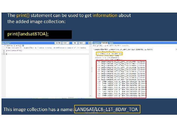
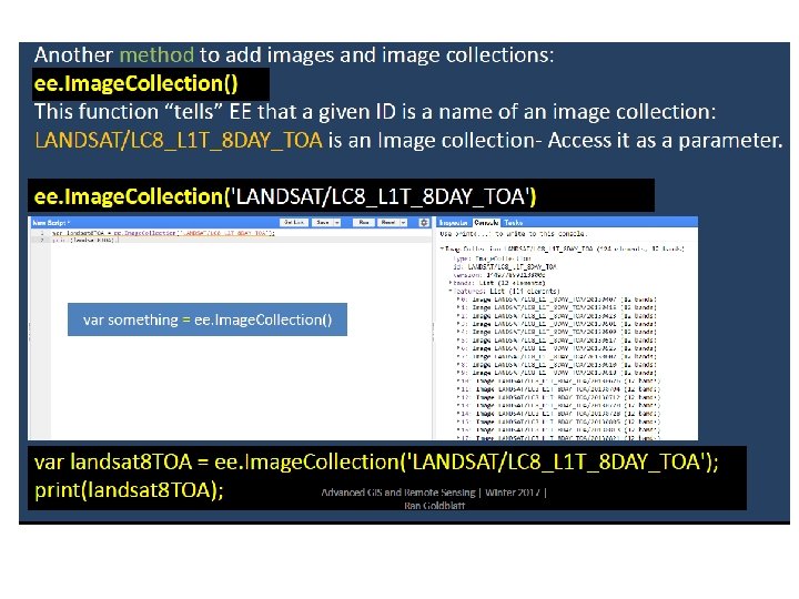
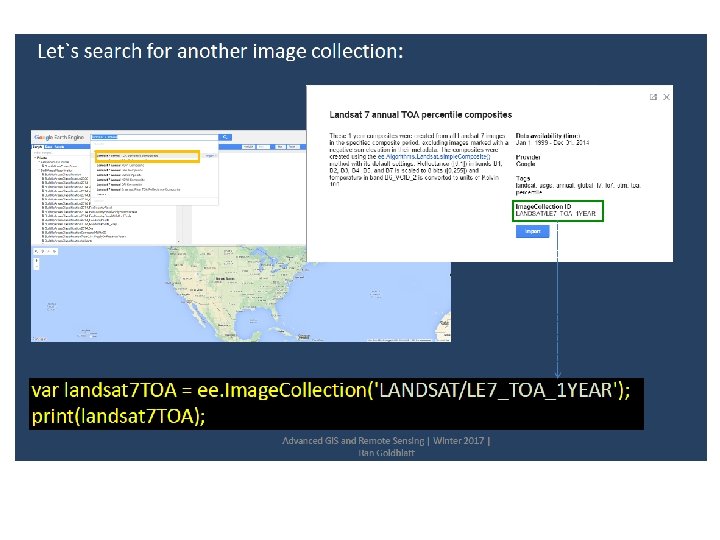
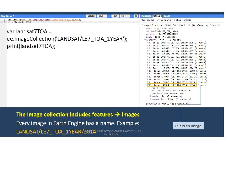
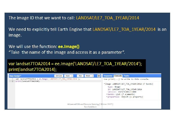
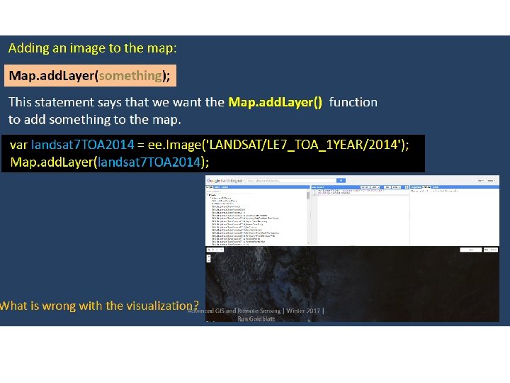
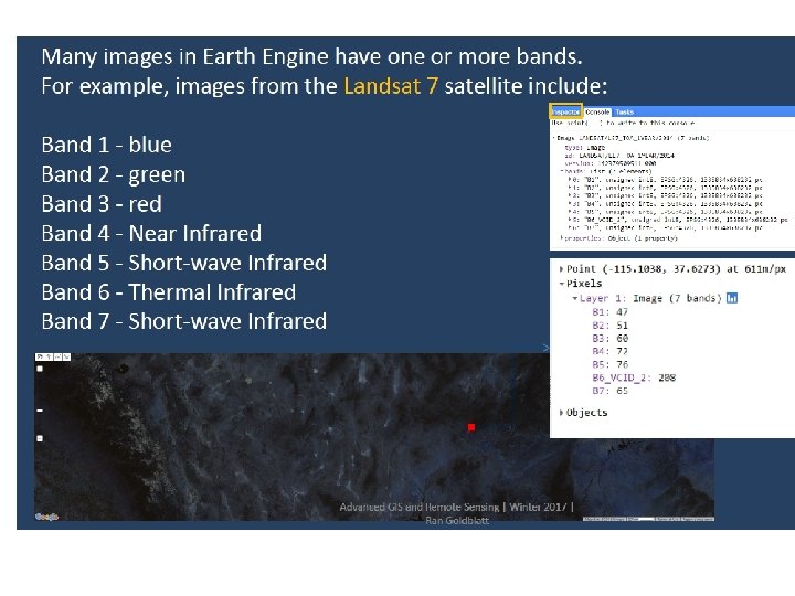
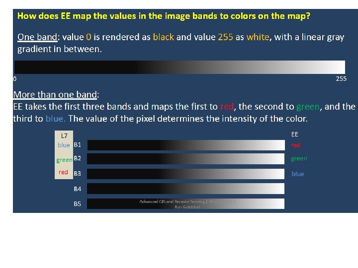
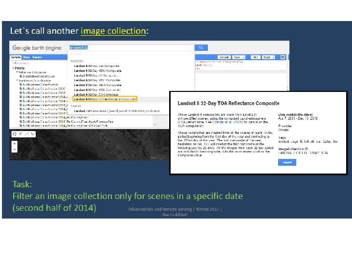
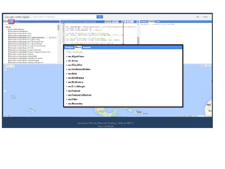
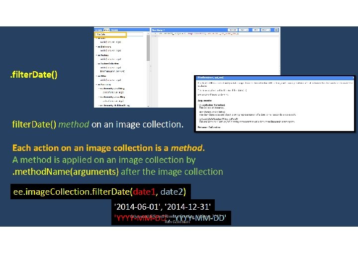
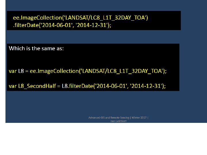
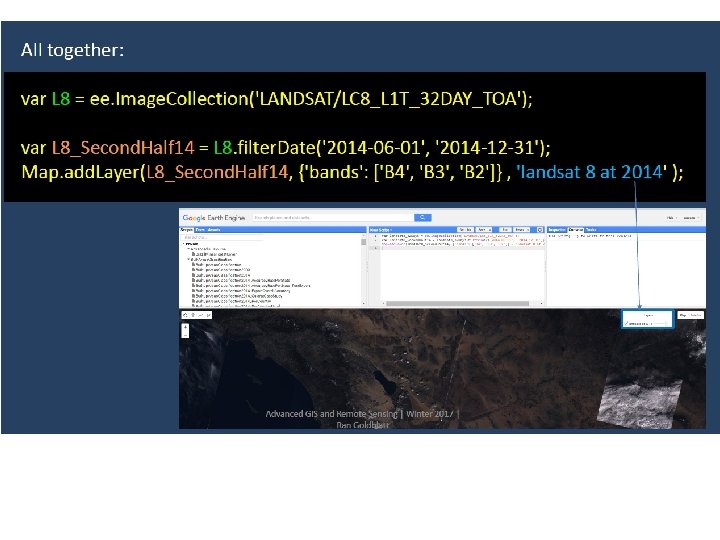
Next explanatory slides are an excerpt from the eetutorial published on the ee-site. • Introductory Remote Sensing Lectures • The materials were prepared by Ran Goldblatt for the Advanced Spatial Analysis class in UC San Diego's School of Global Policy and Strategy and the Center on Global Transformation • https: //developers. google. com/earth-engine/edu#introductory-remote-sensinglectures

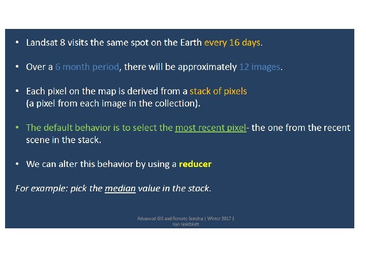
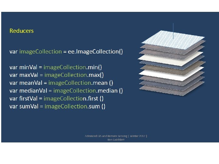
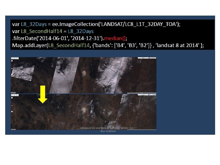
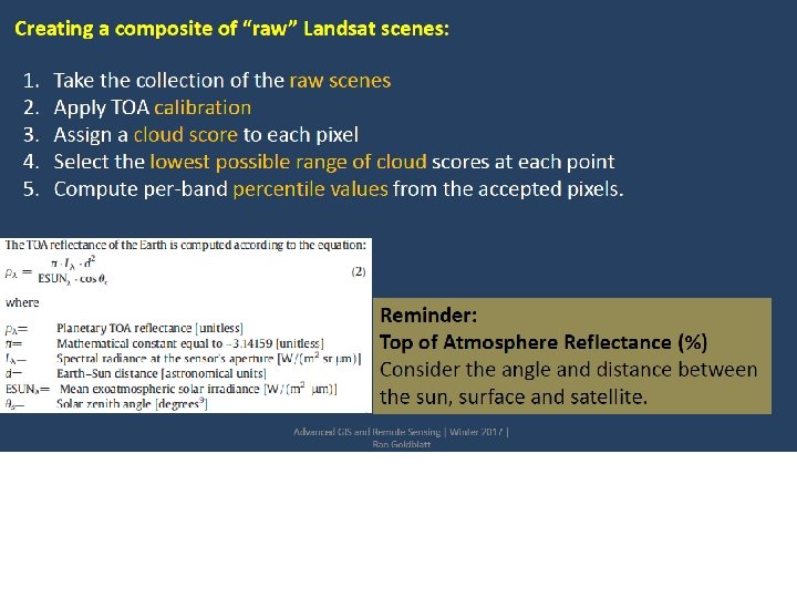
REDUCERS • In the following the reducers are introduced, which have the scope of creating a single image from the analysis of a collection of images.

Temperature conversion

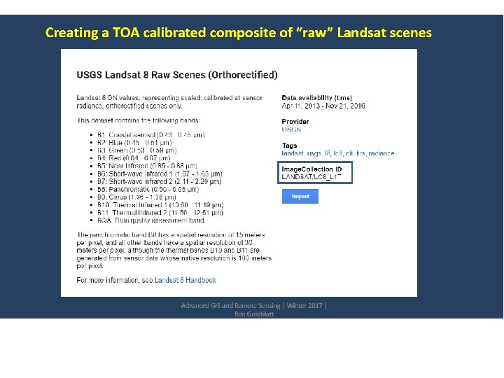
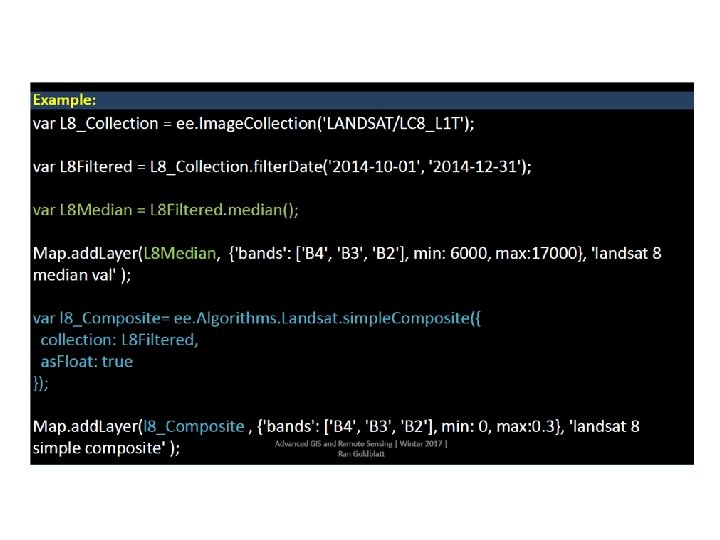
Script 04 • var landsat 8 = ee. Image. Collection("LANDSAT/LC 8_L 1 T_TOA"); • var images = landsat 8. filter. Date('2015 -04 -01', '2015 -04 -06'); • Map. add. Layer(images); Dettagli sulla missione Landsat Vedi documentazione della NASA https: //landsat. gsfc. nasa. gov/landsat-data-continuity-mission/ Esempi di immagini a diverse bande di frequenza: https: //landsat. gsfc. nasa. gov/landsat-8 -bands/

Landsat 8 - summary • • Landsat 8 launched on February 11, 2013, from Vandenberg Air Force Base, California, on an Atlas-V 401 rocket, with the extended payload fairing (EPF) from United Launch Alliance, LLC. The Landsat 8 satellite payload consists of two science instruments—the Operational Land Imager (OLI) and the Thermal Infrared Sensor (TIRS). These two sensors provide seasonal coverage of the global landmass at a spatial resolution of 30 meters (visible, NIR, SWIR); 100 meters (thermal); and 15 meters (panchromatic). Landsat 8 instruments represent an evolutionary advance in technology. OLI improves on past Landsat sensors. OLI is a push-broom sensor with a four-mirror telescope and 12 -bit quantization. OLI collects data for visible, near infrared, and short wave infrared spectral bands as well as a panchromatic band. It has a fiveyear design life. The graphic below compares the OLI spectral bands to Landsat 7′s ETM+ bands. OLI provides two new spectral bands, the coastal band (band 1) and a cirrus cloud band (band 9),

Comparison of spectral bands of Landsat 8 and Landsat 7

Landsat 1 Launch Date: July 23, 1972 Status: expired, January 6, 1978 Sensors: RBV, MSS Altitude: nominally 900 km Inclination: 99. 2° Orbit: polar, sun-synchronous Equatorial Crossing Time: nominally 9: 42 AM mean local time (descending node) • Period of Revolution : 103 minutes; ~14 orbits/day • Repeat Coverage : 18 days • •

Script 04 • var landsat 8 = ee. Image. Collection("LANDSAT/LC 8_L 1 T_TOA"); • var images = landsat 8. filter. Date('2015 -04 -01', '2015 -04 -06'); • Map. add. Layer(images); Per esercizio: variare i periodi temporali Consultare le proprieta’ del database Landsat 8. Caricare un altro database, per esempio sentinel 2 o landsat 7. Confrontare con le proprieta’ di landsat 7. Attenzione a scegliere le date opportune avendo controllato la copertura sulla documentazione.

Script 04 -continua var landsat 8 = ee. Image. Collection("LANDSAT/LC 8_L 1 T_TOA"); var images = landsat 8. filter. Date('2015 -04 -01', '2015 -04 -06'); Map. add. Layer(images); Ispezionare le proprieta’ della figura in scala di grigi nel menu “Inspector” Nell’imagine sono sovrapposte tutte le bande facenti parte della collezione. Nel prossimo script selezioniamo le bande del visibile e dell’infrarosso.