Model Checking Lawrence Chung Safety and Liveness Safety

Model Checking Lawrence Chung

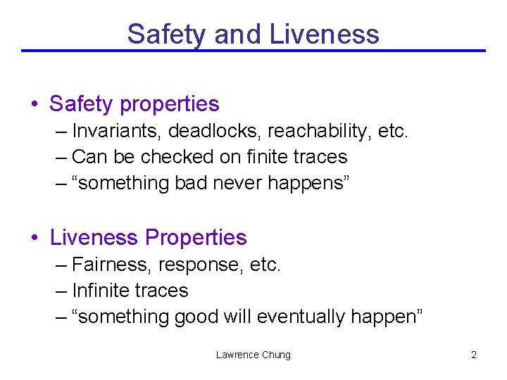
Safety and Liveness • Safety properties – Invariants, deadlocks, reachability, etc. – Can be checked on finite traces – “something bad never happens” • Liveness Properties – Fairness, response, etc. – Infinite traces – “something good will eventually happen” Lawrence Chung 2

Model Checking Process [ Adapted from www. lix. polytechnique. fr/comete/seminar/1 -Model. Checking. ppt] Model Answer: (System Requirements) Specification (System Property) Model Checker M╞ φ Yes, if model satisfies specification Counterexample, otherwise For increasing our confidence in the correctness of the model: q Verification: The model satisfies important system properties q Debugging: Study counter-examples, pinpoint the source of the error, correct the model, and try again Lawrence Chung 3

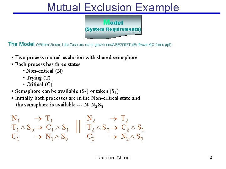
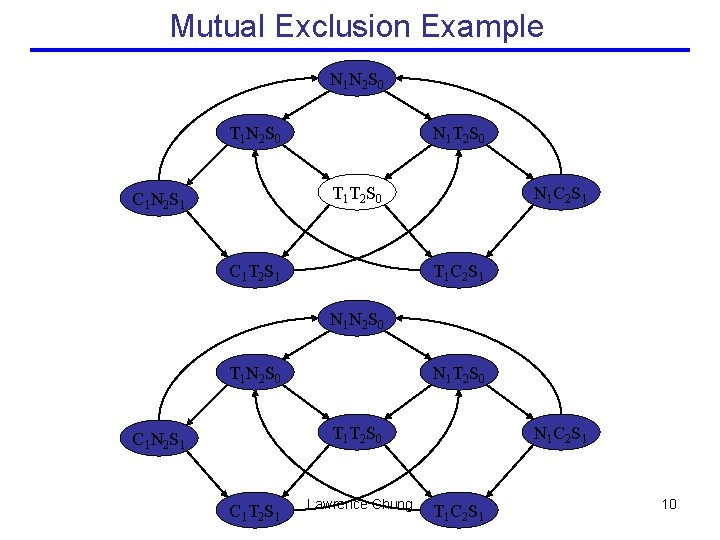
Mutual Exclusion Example Model (System Requirements) The Model (Willem Visser, http: //ase. arc. nasa. gov/visser/ASE 2002 Tut. Software. MC-fonts. ppt) • Two process mutual exclusion with shared semaphore • Each process has three states • Non-critical (N) • Trying (T) • Critical (C) • Semaphore can be available (S 0) or taken (S 1) • Initially both processes are in the Non-critical state and the semaphore is available --- N 1 N 2 S 0 N 1 T 1 S 0 C 1 S 1 C 1 N 1 S 0 || N 2 T 2 S 0 C 2 S 1 C 2 N 2 S 0 Lawrence Chung 4

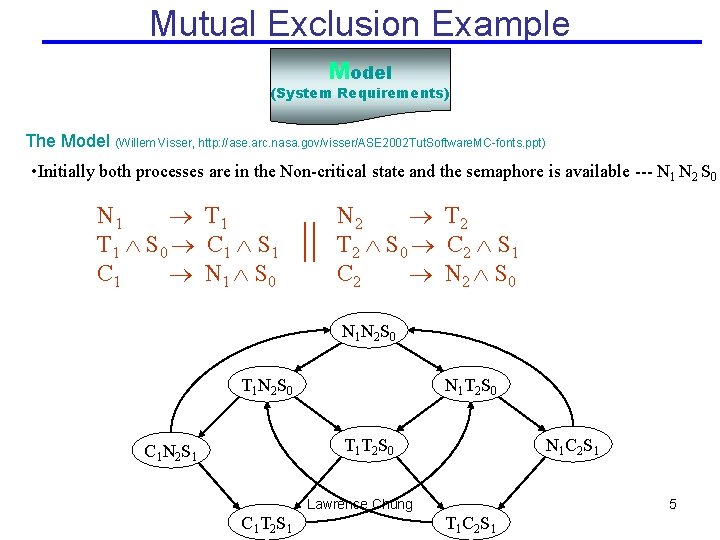
Mutual Exclusion Example Model (System Requirements) The Model (Willem Visser, http: //ase. arc. nasa. gov/visser/ASE 2002 Tut. Software. MC-fonts. ppt) • Initially both processes are in the Non-critical state and the semaphore is available --- N 1 N 2 S 0 N 1 T 1 S 0 C 1 S 1 C 1 N 1 S 0 || N 2 T 2 S 0 C 2 S 1 C 2 N 2 S 0 N 1 N 2 S 0 T 1 N 2 S 0 N 1 T 2 S 0 T 1 T 2 S 0 C 1 N 2 S 1 N 1 C 2 S 1 Lawrence Chung C 1 T 2 S 1 5 T 1 C 2 S 1

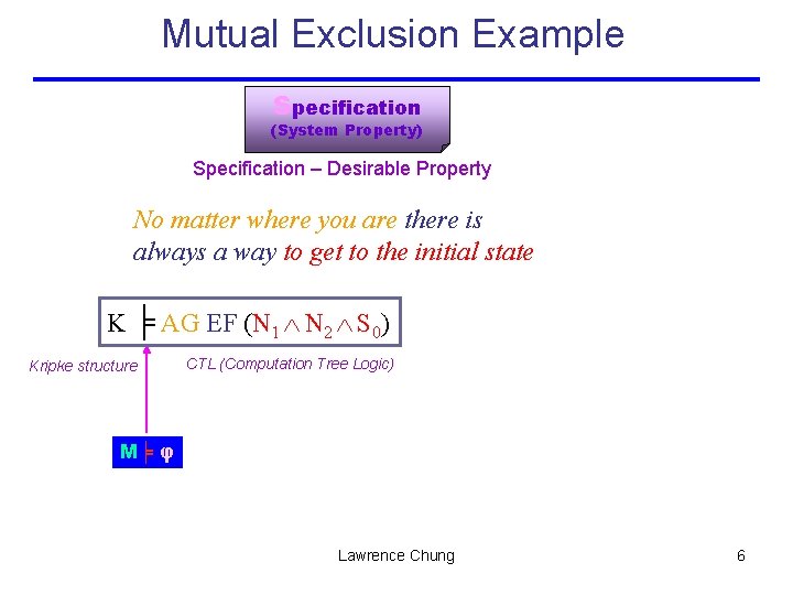
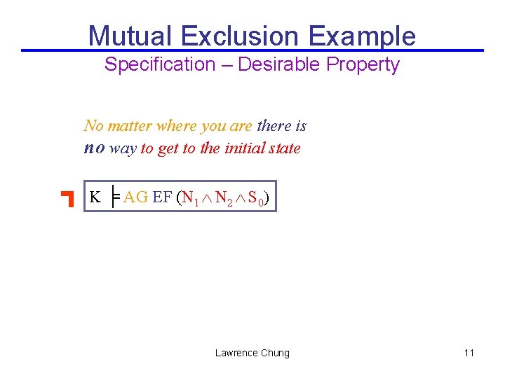
Mutual Exclusion Example Specification (System Property) Specification – Desirable Property No matter where you are there is always a way to get to the initial state K ╞ AG EF (N 1 N 2 S 0) Kripke structure CTL (Computation Tree Logic) M╞ φ Lawrence Chung 6

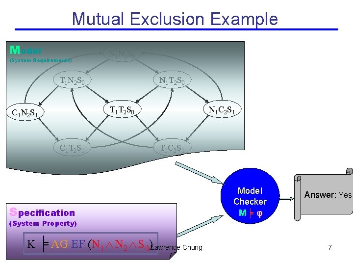
Mutual Exclusion Example Model (System Requirements) N 1 N 2 S 0 T 1 N 2 S 0 N 1 T 2 S 0 T 1 T 2 S 0 C 1 N 2 S 1 C 1 T 2 S 1 N 1 C 2 S 1 T 1 C 2 S 1 Specification (System Property) K ╞ AG EF (N 1 N 2 S 0)Lawrence Chung Model Checker M╞ φ Answer: Yes 7

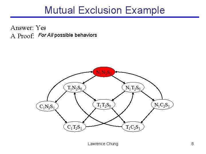
Mutual Exclusion Example Answer: Yes A Proof: For All possible behaviors N 1 N 2 S 0 T 1 N 2 S 0 N 1 T 2 S 0 T 1 T 2 S 0 C 1 N 2 S 1 C 1 T 2 S 1 N 1 C 2 S 1 T 1 C 2 S 1 Lawrence Chung 8

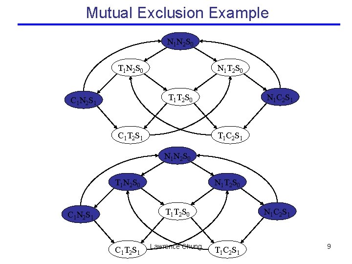
Mutual Exclusion Example N 1 N 2 S 0 T 1 N 2 S 0 N 1 T 2 S 0 T 1 T 2 S 0 C 1 N 2 S 1 C 1 T 2 S 1 N 1 C 2 S 1 T 1 C 2 S 1 N 2 S 0 T 1 N 2 S 0 N 1 T 2 S 0 T 1 T 2 S 0 C 1 N 2 S 1 C 1 T 2 S 1 Lawrence Chung N 1 C 2 S 1 T 1 C 2 S 1 9

Mutual Exclusion Example N 1 N 2 S 0 T 1 N 2 S 0 N 1 T 2 S 0 T 1 T 2 S 0 C 1 N 2 S 1 C 1 T 2 S 1 N 1 C 2 S 1 T 1 C 2 S 1 N 2 S 0 T 1 N 2 S 0 N 1 T 2 S 0 T 1 T 2 S 0 C 1 N 2 S 1 C 1 T 2 S 1 Lawrence Chung N 1 C 2 S 1 T 1 C 2 S 1 10

Mutual Exclusion Example Specification – Desirable Property No matter where you are there is no way to get to the initial state ⌐ K ╞ AG EF (N 1 N 2 S 0) Lawrence Chung 11

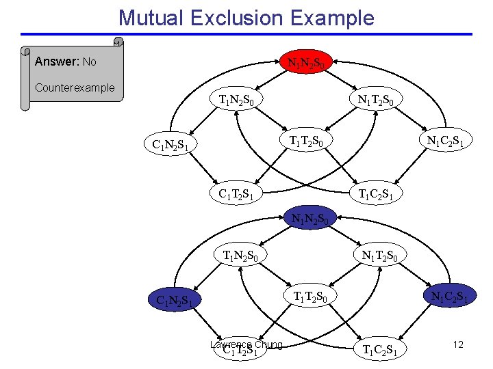
Mutual Exclusion Example Answer: No N 1 N 2 S 0 Counterexample T 1 N 2 S 0 N 1 T 2 S 0 T 1 T 2 S 0 C 1 N 2 S 1 C 1 T 2 S 1 N 1 C 2 S 1 T 1 C 2 S 1 N 2 S 0 T 1 N 2 S 0 N 1 T 2 S 0 T 1 T 2 S 0 C 1 N 2 S 1 Lawrence Chung C 1 T 2 S 1 N 1 C 2 S 1 T 1 C 2 S 1 12

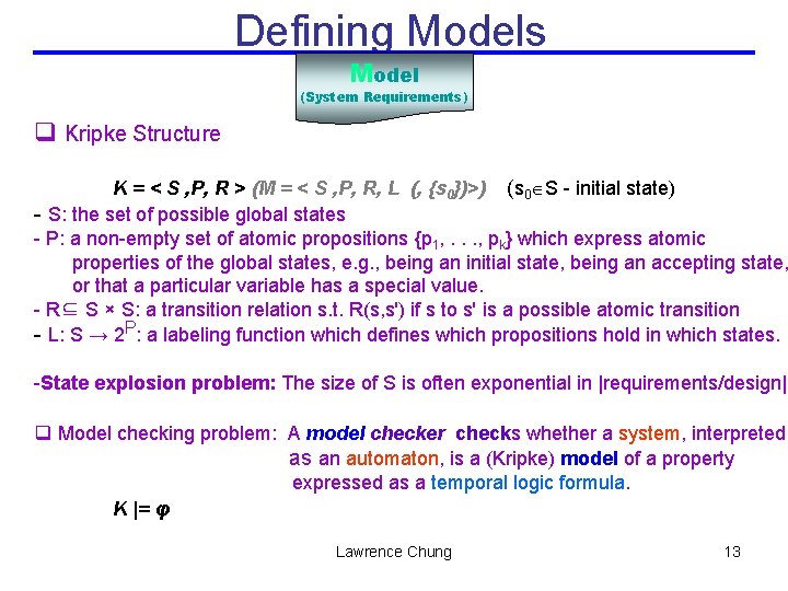
Defining Models Model (System Requirements) q Kripke Structure K = < S , P, R > (M = < S , P, R, L (, {s 0})>) (s 0 S - initial state) - S: the set of possible global states - P: a non-empty set of atomic propositions {p 1, . . . , pk} which express atomic properties of the global states, e. g. , being an initial state, being an accepting state, or that a particular variable has a special value. - R⊆ S × S: a transition relation s. t. R(s, s') if s to s' is a possible atomic transition - L: S → 2 P: a labeling function which defines which propositions hold in which states. -State explosion problem: The size of S is often exponential in |requirements/design|. q Model checking problem: A model checker checks whether a system, interpreted as an automaton, is a (Kripke) model of a property expressed as a temporal logic formula. K |= φ Lawrence Chung 13

Defining Models q For a complex real-life control systems Extended Finite State Machine (EFSM) - FSM with a way to -modularize the requirements to view them at different levels of detail -combine requirements (or design) of components - state variables and facilities in guards on transitions. Lawrence Chung 14

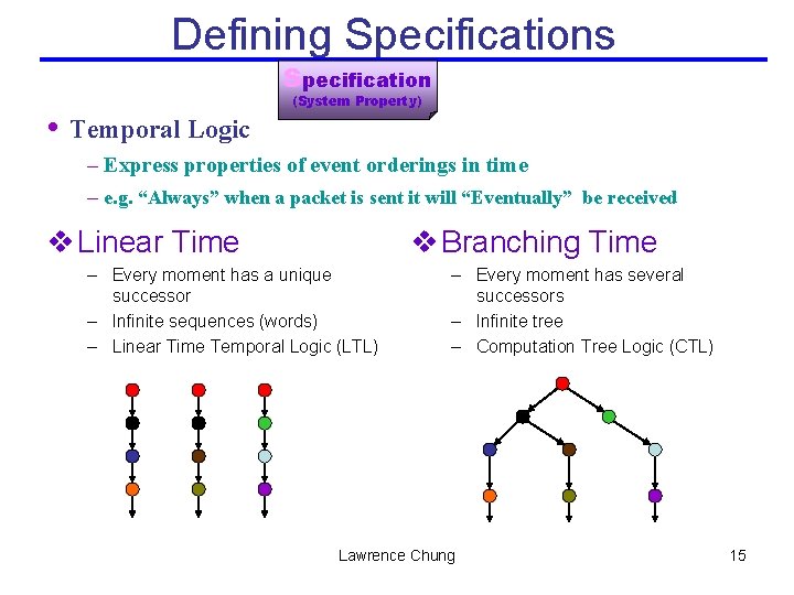
Defining Specifications Specification • Temporal Logic (System Property) – Express properties of event orderings in time – e. g. “Always” when a packet is sent it will “Eventually” be received v Linear Time v Branching Time – Every moment has a unique successor – Infinite sequences (words) – Linear Time Temporal Logic (LTL) – Every moment has several successors – Infinite tree – Computation Tree Logic (CTL) Lawrence Chung 15

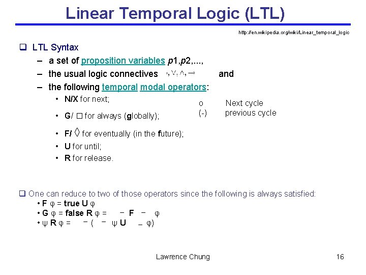
Linear Temporal Logic (LTL) http: //en. wikipedia. org/wiki/Linear_temporal_logic q LTL Syntax – a set of proposition variables p 1, p 2, . . . , – the usual logic connectives and – the following temporal modal operators: • N/X for next; • G/ □ for always (globally); o Next cycle (-) previous cycle • F/ ◊ for eventually (in the future); • U for until; • R for release. q One can reduce to two of those operators since the following is always satisfied: • F φ = true U φ • G φ = false R φ = F φ • ψ R φ = ( ψ U φ) Lawrence Chung 16

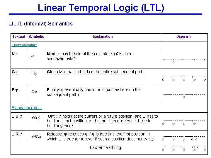
Linear Temporal Logic (LTL) q. LTL (Informal) Semantics Textual Symbolic Explanation Diagram Unary operators: N φ Next: φ has to hold at the next state. (X is used synonymously. ) G φ Globally: φ has to hold on the entire subsequent path. F φ Finally: φ eventually has to hold (somewhere on the subsequent path). Binary operators: ψ U φ Until: φ holds at the current or a future position, and ψ has to hold until that position. At that position ψ does not have to hold any more. ψ R φ Release: ψ releases φ if φ is true until the first position in which ψ is true (or forever if such a position does not exist). Lawrence Chung 17

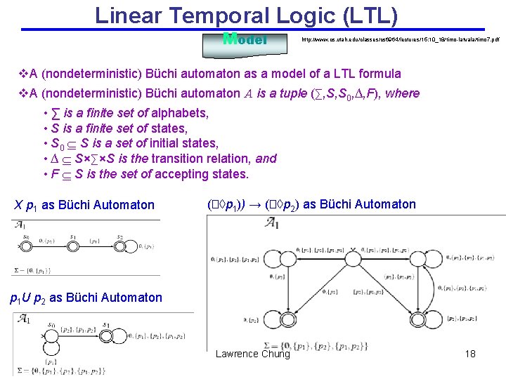
Linear Temporal Logic (LTL) Model http: //www. cs. utah. edu/classes/cs 6964/lectures/15: 10_18/timo-latvala/timo 7. pdf v. A (nondeterministic) Büchi automaton as a model of a LTL formula v. A (nondeterministic) Büchi automaton A is a tuple (∑, S, S 0, ∆, F), where • ∑ is a finite set of alphabets, • S is a finite set of states, • S 0 S is a set of initial states, • ∆ S×∑×S is the transition relation, and • F S is the set of accepting states. X p 1 as Büchi Automaton (�◊p 1)) → (�◊p 2) as Büchi Automaton p 1 U p 2 as Büchi Automaton Lawrence Chung 18

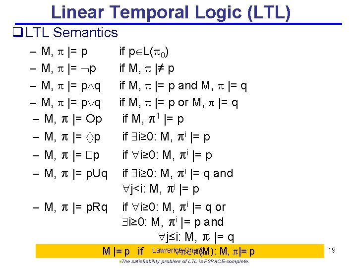
Linear Temporal Logic (LTL) q LTL Semantics – M, |= p q – M, |= Op if p L( 0) if M, |≠ p if M, |= p and M, |= q if M, |= p or M, |= q if M, 1 |= p – M, |= p if i≥ 0: M, i |= p – M, |= �p if i≥ 0: M, i |= p – M, |= p. Uq if i≥ 0: M, i |= q and j<i: M, j |= p – M, |= p. Rq if i≥ 0: M, i |= q or i≥ 0: M, i |= p and j≤i: M, j |= q M |= p if n. The Lawrence Chung (M): M, |= p satisfiability problem of LTL is PSPACE-complete. 19

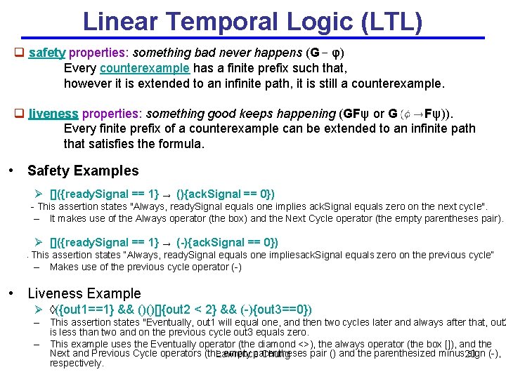
Linear Temporal Logic (LTL) q safety properties: something bad never happens (G φ) Every counterexample has a finite prefix such that, however it is extended to an infinite path, it is still a counterexample. q liveness properties: something good keeps happening (GFψ or G Fψ)). Every finite prefix of a counterexample can be extended to an infinite path that satisfies the formula. • Safety Examples Ø []({ready. Signal == 1} → (){ack. Signal == 0}) - This assertion states "Always, ready. Signal equals one implies ack. Signal equals zero on the next cycle". – It makes use of the Always operator (the box) and the Next Cycle operator (the empty parentheses pair). Ø []({ready. Signal == 1} → (-){ack. Signal == 0}) This assertion states “Always, ready. Signal equals one impliesack. Signal equals zero on the previous cycle“ – Makes use of the previous cycle operator (-) - • Liveness Example Ø ◊({out 1==1} && ()()[]{out 2 < 2} && (-){out 3==0}) – This assertion states "Eventually, out 1 will equal one, and then two cycles later and always after that, out 2 is less than two and on the previous cycle out 3 equals zero. – This example uses the Eventually operator (the diamond <>), the always operator (the box []), and the Next and Previous Cycle operators (the empty parentheses pair () and the parenthesized minus sign (-), Lawrence Chung 20 respectively.

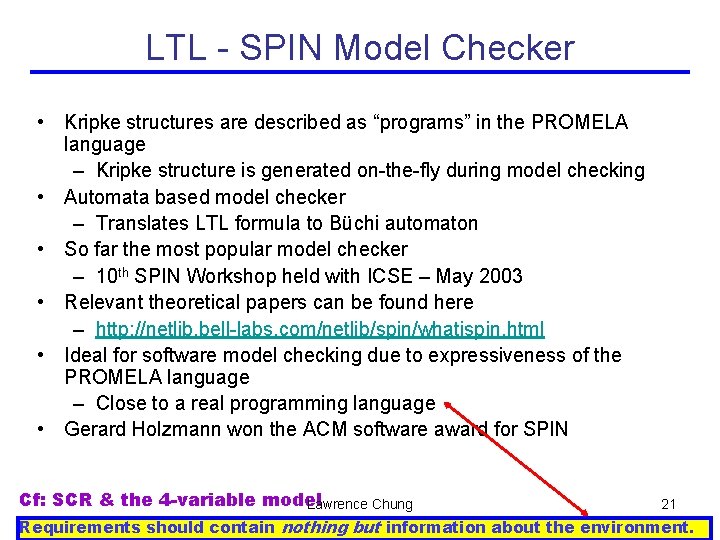
LTL - SPIN Model Checker • Kripke structures are described as “programs” in the PROMELA language – Kripke structure is generated on-the-fly during model checking • Automata based model checker – Translates LTL formula to Büchi automaton • So far the most popular model checker – 10 th SPIN Workshop held with ICSE – May 2003 • Relevant theoretical papers can be found here – http: //netlib. bell-labs. com/netlib/spin/whatispin. html • Ideal for software model checking due to expressiveness of the PROMELA language – Close to a real programming language • Gerard Holzmann won the ACM software award for SPIN Cf: SCR & the 4 -variable model Lawrence Chung 21 Requirements should contain nothing but information about the environment.

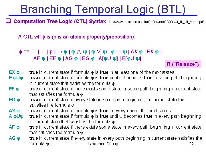
Branching Temporal Logic (BTL) q Computation Tree Logic (CTL) Syntax http: //www. cs. ucl. ac. uk/staff/J. Bowen/GS 03/w 3_l 1_ctl_notes. pdf A CTL wff ϕ is (p is an atomic property/proposition): ϕ : : = ⊤ | ⊥ | p | ￢ φ | φ ∧ ψ | φ ∨ ψ | φ → ψ | AX φ | EX φ | AF φ | EF φ | AG φ | EG φ | A[φU ψ] | E[φU ψ] R (‘‘Release’’) EX φ E φUψ EF φ EG φ AX φ A φUψ AF φ AG φ true in current state if formula φ is true in at least one of the next states true in current state if formula φ is true until ψ becomes true in some path beginning in current state that satisfies the formula φ true in current state if there exists some state in some path beginning in current state that satisfies the formula φ true in current state if every state in some path beginning in current state that satisfies the formula φ true in current state if formula φ is true in every one of the next states true in current state if formula φ is true until ψ becomes true in every path beginning in current state that satisfies the formula φ true in current state if there exists some state in every path beginning in current state that satisfies the formula φ true in current state if every state in every path beginning in current state satisfies the formula φ Lawrence Chung 22

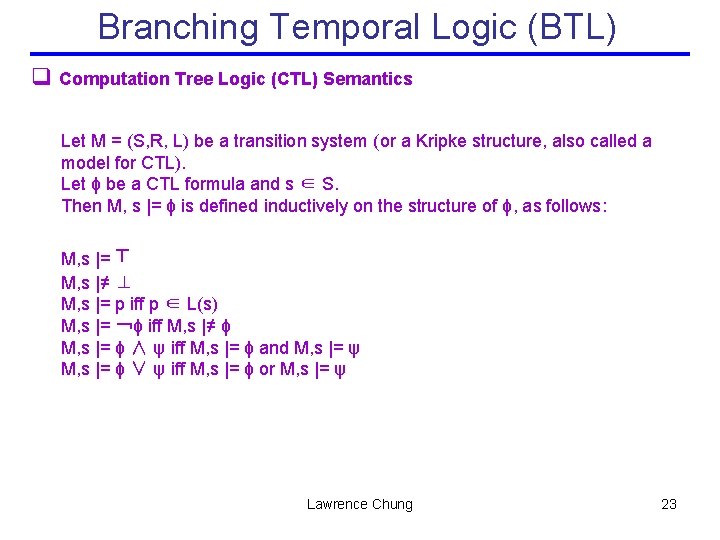
Branching Temporal Logic (BTL) q Computation Tree Logic (CTL) Semantics Let M = (S, R, L) be a transition system (or a Kripke structure, also called a model for CTL). Let ϕ be a CTL formula and s ∈ S. Then M, s |= ϕ is defined inductively on the structure of ϕ, as follows: M, s |= ⊤ M, s |≠ ⊥ M, s |= p iff p ∈ L(s) M, s |= ￢ϕ iff M, s |≠ ϕ M, s |= ϕ ∧ ψ iff M, s |= ϕ and M, s |= ψ M, s |= ϕ ∨ ψ iff M, s |= ϕ or M, s |= ψ Lawrence Chung 23

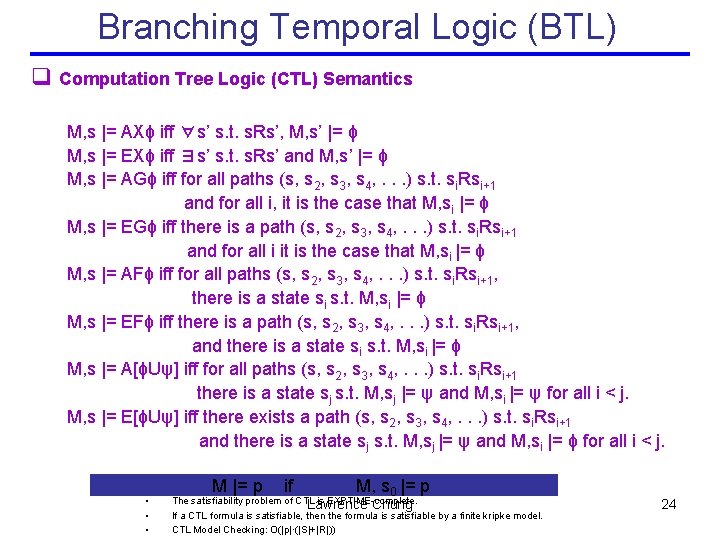
Branching Temporal Logic (BTL) q Computation Tree Logic (CTL) Semantics M, s |= AXϕ iff ∀s’ s. t. s. Rs’, M, s’ |= ϕ M, s |= EXϕ iff ∃s’ s. t. s. Rs’ and M, s’ |= ϕ M, s |= AGϕ iff for all paths (s, s 2, s 3, s 4, . . . ) s. t. si. Rsi+1 and for all i, it is the case that M, si |= ϕ M, s |= EGϕ iff there is a path (s, s 2, s 3, s 4, . . . ) s. t. si. Rsi+1 and for all i it is the case that M, si |= ϕ M, s |= AFϕ iff for all paths (s, s 2, s 3, s 4, . . . ) s. t. si. Rsi+1, there is a state si s. t. M, si |= ϕ M, s |= EFϕ iff there is a path (s, s 2, s 3, s 4, . . . ) s. t. si. Rsi+1, and there is a state si s. t. M, si |= ϕ M, s |= A[ϕUψ] iff for all paths (s, s 2, s 3, s 4, . . . ) s. t. si. Rsi+1 there is a state sj s. t. M, sj |= ψ and M, si |= ψ for all i < j. M, s |= E[ϕUψ] iff there exists a path (s, s 2, s 3, s 4, . . . ) s. t. si. Rsi+1 and there is a state sj s. t. M, sj |= ψ and M, si |= ϕ for all i < j. • • • M |= p if M, s 0 |= p The satisfiability problem of CTL is EXPTIME-complete. Lawrence Chung If a CTL formula is satisfiable, then the formula is satisfiable by a finite kripke model. CTL Model Checking: O(|p|·(|S|+|R|)) 24

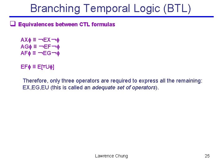
Branching Temporal Logic (BTL) q Equivalences between CTL formulas AXϕ ≡ ￢EX￢ϕ AGϕ ≡ ￢EF￢ϕ AFϕ ≡ ￢EG￢ϕ EFϕ ≡ E[⊤Uϕ] Therefore, only three operators are required to express all the remaining: EX, EG, EU (this is called an adequate set of operators). Lawrence Chung 25

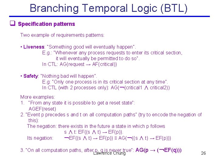
Branching Temporal Logic (BTL) q Specification patterns Two example of requirements patterns: • Liveness: “Something good will eventually happen”. E. g. : “Whenever any process requests to enter its critical section, it will eventually be permitted to do so”. In CTL: AG(request → AF(critical)) • Safety: “Nothing bad will happen”. E. g: “Only one process is in its critical section at any time”. In CTL (with 2 processes only): AG(￢(critical 1 ∧ critical 2)) More examples: 1. “From any state it is possible to get a reset state”: AGEF(reset) 2. “Event p precedes s and t on all computation paths” (try to encode the negation of this): The negation: there exists in the future a state in which p follows s ∧ t: EF((s ∧ t) → EF(p)). Its negation: ￢EF((s ∧ t) → EF(p)) ≡ AG(￢((s ∧ t) → EF(p))) 3. “On all computation paths, after p, q is never true”: AG(p → (￢EF(q))) Lawrence Chung 26

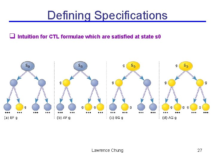
Defining Specifications q Intuition for CTL formulae which are satisfied at state s 0 Lawrence Chung 27

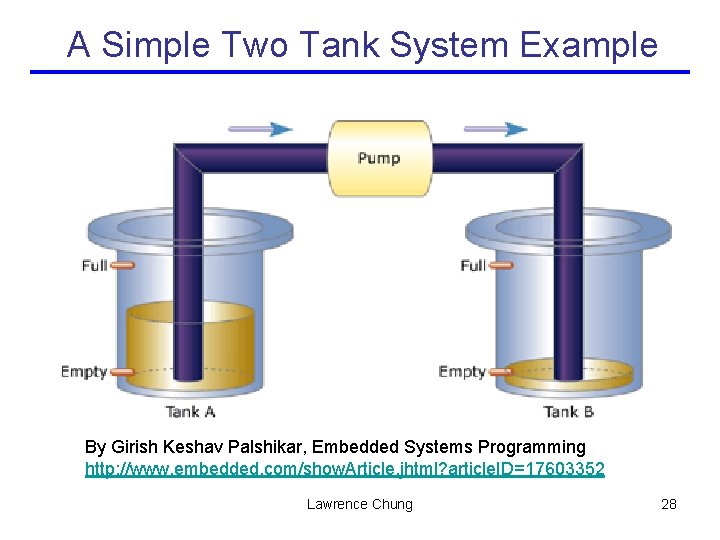
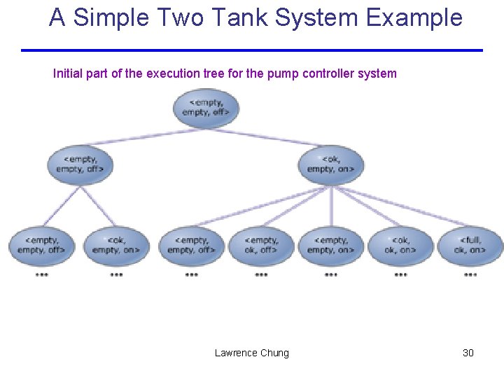
A Simple Two Tank System Example By Girish Keshav Palshikar, Embedded Systems Programming http: //www. embedded. com/show. Article. jhtml? article. ID=17603352 Lawrence Chung 28

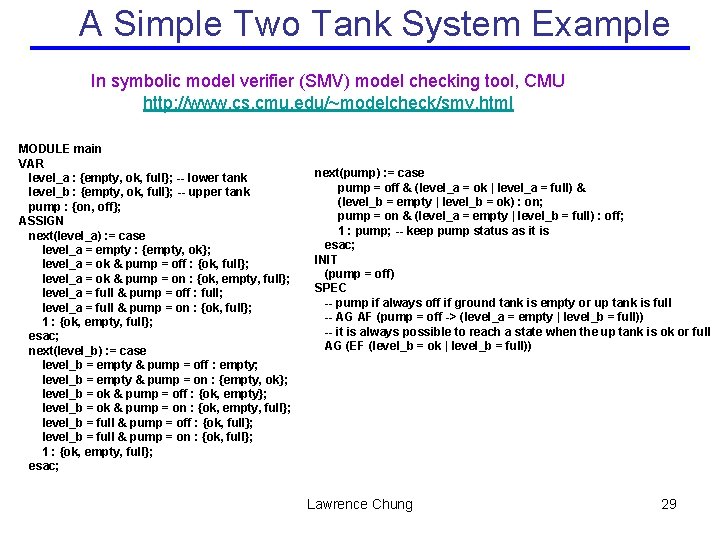
A Simple Two Tank System Example In symbolic model verifier (SMV) model checking tool, CMU http: //www. cs. cmu. edu/~modelcheck/smv. html MODULE main VAR level_a : {empty, ok, full}; -- lower tank level_b : {empty, ok, full}; -- upper tank pump : {on, off}; ASSIGN next(level_a) : = case level_a = empty : {empty, ok}; level_a = ok & pump = off : {ok, full}; level_a = ok & pump = on : {ok, empty, full}; level_a = full & pump = off : full; level_a = full & pump = on : {ok, full}; 1 : {ok, empty, full}; esac; next(level_b) : = case level_b = empty & pump = off : empty; level_b = empty & pump = on : {empty, ok}; level_b = ok & pump = off : {ok, empty}; level_b = ok & pump = on : {ok, empty, full}; level_b = full & pump = off : {ok, full}; level_b = full & pump = on : {ok, full}; 1 : {ok, empty, full}; esac; next(pump) : = case pump = off & (level_a = ok | level_a = full) & (level_b = empty | level_b = ok) : on; pump = on & (level_a = empty | level_b = full) : off; 1 : pump; -- keep pump status as it is esac; INIT (pump = off) SPEC -- pump if always off if ground tank is empty or up tank is full -- AG AF (pump = off -> (level_a = empty | level_b = full)) -- it is always possible to reach a state when the up tank is ok or full AG (EF (level_b = ok | level_b = full)) Lawrence Chung 29

A Simple Two Tank System Example Initial part of the execution tree for the pump controller system Lawrence Chung 30

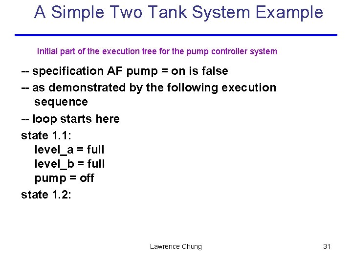
A Simple Two Tank System Example Initial part of the execution tree for the pump controller system -- specification AF pump = on is false -- as demonstrated by the following execution sequence -- loop starts here state 1. 1: level_a = full level_b = full pump = off state 1. 2: Lawrence Chung 31

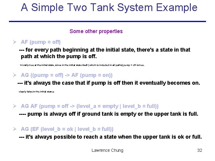
A Simple Two Tank System Example Some other properties Ø AF (pump = off) --- for every path beginning at the initial state, there's a state in that path at which the pump is off. trivially true at the initial state, since in the initial state itself (which is included in all paths) pump = off is true. Ø AG ((pump = off) -> AF (pump = on)) --- it's always the case that if pump is off then it eventually becomes on. clearly false in the initial state. Ø AG AF (pump = off -> (level_a = empty | level_b = full)) ---- pump is always off if ground tank is empty or the upper tank is full. Ø AG (EF (level_b = ok | level_b = full)) --- it's always possible to reach a state when the upper tank is ok or full. Lawrence Chung 32

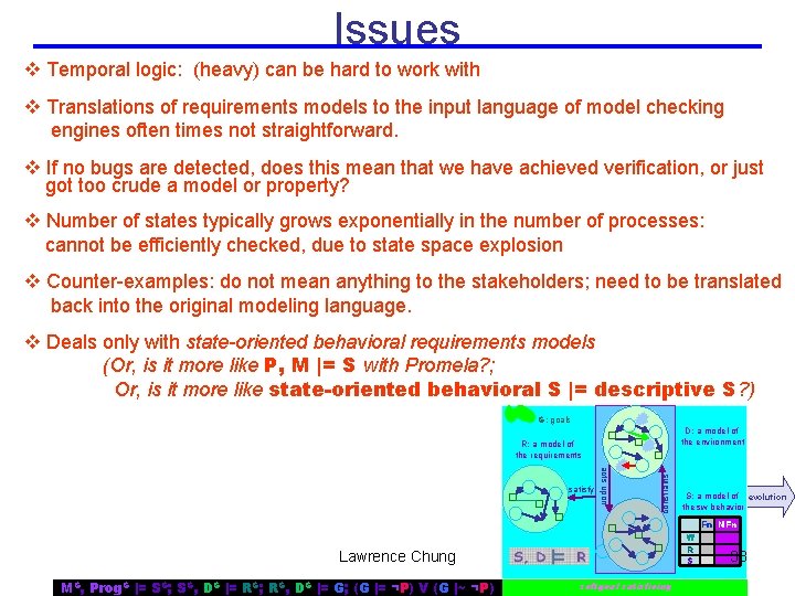
Issues v Temporal logic: (heavy) can be hard to work with v Translations of requirements models to the input language of model checking engines often times not straightforward. v If no bugs are detected, does this mean that we have achieved verification, or just got too crude a model or property? v Number of states typically grows exponentially in the number of processes: cannot be efficiently checked, due to state space explosion v Counter-examples: do not mean anything to the stakeholders; need to be translated back into the original modeling language. v Deals only with state-oriented behavioral requirements models (Or, is it more like P, M |= S with Promela? ; Or, is it more like state-oriented behavioral S |= descriptive S? ) G: goals D: a model of the environment acts upon satisfy constrains R: a model of the requirements S: a model of evolution the sw behavior Fn NFn W R S Lawrence Chung MG, Prog. G |= SG; SG, DG |= RG; RG, DG |= G; (G |= ¬P) V (G |~ ¬P) softgoal satisficing 33

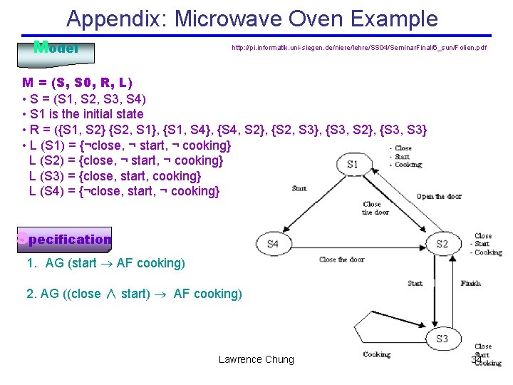
Appendix: Microwave Oven Example Model http: //pi. informatik. uni-siegen. de/niere/lehre/SS 04/Seminar. Final/6_sun/Folien. pdf M = (S, S 0, R, L) • S = (S 1, S 2, S 3, S 4) • S 1 is the initial state • R = ({S 1, S 2} {S 2, S 1}, {S 1, S 4}, {S 4, S 2}, {S 2, S 3}, {S 3, S 2}, {S 3, S 3} • L (S 1) = {¬close, ¬ start, ¬ cooking} L (S 2) = {close, ¬ start, ¬ cooking} L (S 3) = {close, start, cooking} L (S 4) = {¬close, start, ¬ cooking} Specification 1. AG (start AF cooking) 2. AG ((close ∧ start) AF cooking) Lawrence Chung 34

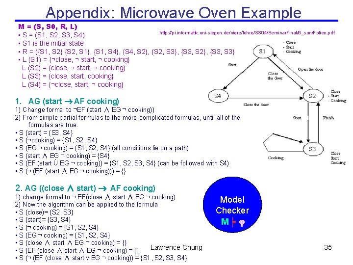
Appendix: Microwave Oven Example M = (S, S 0, R, L) http: //pi. informatik. uni-siegen. de/niere/lehre/SS 04/Seminar. Final/6_sun/Folien. pdf • S = (S 1, S 2, S 3, S 4) • S 1 is the initial state • R = ({S 1, S 2} {S 2, S 1}, {S 1, S 4}, {S 4, S 2}, {S 2, S 3}, {S 3, S 2}, {S 3, S 3} • L (S 1) = {¬close, ¬ start, ¬ cooking} L (S 2) = {close, ¬ start, ¬ cooking} L (S 3) = {close, start, cooking} L (S 4) = {¬close, start, ¬ cooking} 1. AG (start AF cooking) 1) Change formal to ¬EF (start ∧ EG ¬ cooking)) 2) From simple partial formulas to the more complicated formulas, until all of the formulas are true. • S (start) = {S 3, S 4} • S (¬cooking) = {S 1, S 2, S 4} • S (EG ¬ cooking) = {S 1, S 2, S 4} (all conditions lie on a path) • S (start ∧ EG ¬ cooking) = {S 4} • S (EF (start Ù EG ¬ cooking)) = {S 1, S 2, S 3, S 4} (can be followed with S 4) • S (¬ (EF (start ∧ EG ¬ cooking))) = {} 2. AG ((close ∧ start) AF cooking) 1) change formal to ¬ EF(close ∧ start ∧ EG ¬ cooking) 2) Now the algorithm can be applied to the formula • S (close)= {S 2, S 3} • S (start)= {S 3, S 4} • S (¬ cooking) = {S 1, S 2, S 4} • S (EG ¬ cooking) = {S 1, S 2, S 4} • S (close ∧ start ∧ EG ¬ cooking) = {} Lawrence Chung • S (EF (close ∧ start ∧ EG ¬ cooking) = {} • S (¬ (EF (close ∧ start v EG ¬ cooking)) = {S 1, S 2, S 3, S 4} Model Checker M╞ φ 35

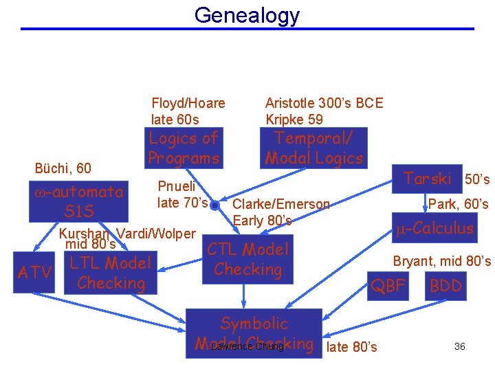
Genealogy Floyd/Hoare late 60 s Büchi, 60 Logics of Programs w-automata S 1 S Pnueli late 70’s Kurshan Vardi/Wolper mid 80’s ATV LTL Model Checking Aristotle 300’s BCE Kripke 59 Temporal/ Modal Logics Tarski 50’s Clarke/Emerson Early 80’s CTL Model Checking Park, 60’s m-Calculus Bryant, mid 80’s QBF Symbolic Model Checking late 80’s Lawrence Chung BDD 36