Mesoscopic quantum measurements D V Averin Department of

Mesoscopic quantum measurements D. V. Averin Department of Physics and Astronomy, SUNY, Stony Brook

Outline 1. Introduction: Josephson junction qubits: 2. - Coulomb blockade of Cooper pair tunneling; 3. - coherent oscillations of two coupled charge qubits; 4. - variable electrostatic transformer for controlled coupling. 2. Quantum measurement problem. 3. Linear measurements. 4. Quadratic measurements and active suppression of dephasing in Josephson junction qubits. Collaboration: Ch. Bruder, R. Fazio, A. N. Korotkov, W. Mao, R. Ruskov Support: ARDA, AFOSR, NSF

Quantum dynamics of Josephson junctions • Superconductor can be thought of as a BEC of Cooper pairs: one single-particle state occupied with macroscopic number of particles. The phase φ and the number of particles n are conjugate quantum variables (Anderson, 64; Ivanchenko, Zil’berman, 65): n, =i. This relation describes dynamics of addition or removal of particles to/from the condensate.

• This dynamics manifests itself most directly in Josephson tunnel junctions, and was studied as an example of macroscopic quantum dynamics (Leggett, 80). • If quantum fluctuations of phase φ become large, junction behavior can be described as a semiclassical dynamics of charge that leads to controlled transfer of individual Cooper pairs (Averin, Zorin, Likharev, 1985).

Charge qubits For EJ <<EC and q≈1/2, the charge tunneling dynamics in an isolated individual junction is directly reduced to the two-state form.

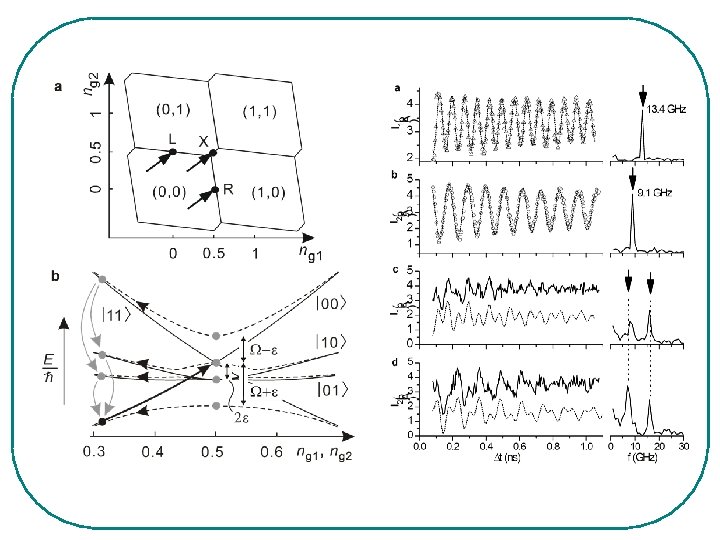
Two coupled charge qubits En 1 n 2 = Ec 1(ng 1–n 1)² + Ec 2(ng 2–n 2)² + +Em(ng 1–n 1)(ng 2–n 2), Em = e²Cm/(CΣ 1 CΣ 2 – Cm 2) Yu. A. Pashkin et al. , Nature 421, 823 (2003).

Variable electrostatic transformer: controlled coupling of charge qubits Equivalent circuit of the variable electrostatic transformer: Gate-controlled qubit coupling: coupling capacitance: D. V. A. and C. Bruder, cond-mat/0304166.

Coupling strength: Charging diagram demonstrates transition from positive to negative coupling

Quantum measurement problem The process of quantum measurement establishes correlations between the states of the measured system and the states of ``macroscopic’’ detector. with probability - ``wave function collapse’’ In the mesoscopic regime, both the detector and the measured systems are of the same ``size’’. In addition, there are new simple quantum ``paradoxes’’. For instance, measurement of the charge qubit leads to changes in a, b and therefore to transfer of charge (for weak measurements, gradual) even if the tunneling is completely suppressed!

Linear quantum measurements Linear-response theory enables one to develop quantitative description of the quantum measurement process with an arbitrary detector provided that it satisfies some general conditions: • the detector/system coupling is weak so that the detector’s response is linear; • the detector is in the stationary state; • the response is instantaneous. D. V. A. , cond-mat/00044364, cond-mat/0010052, and to be published. S. Pilgram and M. Büttiker, PRL 89, 200401 (2002). A. A. Clerk, S. M. Girvin, and A. D. Stone, cond-mat/0211001.

FDT analog for quantum measurements where λ is the linear response coefficient of the detector, Sf and Sq are the low-frequency spectral densities of the, respectively, backaction and output noise, Re. Sfq is the classical part of their crosscorrelator. This inequality shows that finite response coefficient implies that noise generated by the detector is non-vanishing. Although it was obtained from the linear-response theory, it has broader meaning in that it characterizes the efficiency of the trade-off between the information acquisition by the detector and back-action dephasing of the measured system. The detector that satisfies this inequality as equality is called ``ideal’’ or ``quantum-limited’’.

Information/back-action trade-off in quantum measurements Qualitatively, dynamics of the measurement process consists of information acquisition by the detector and back-action dephasing of the measured system. The trade-off between them has the simplest form for measurements of the static system with HS=0. Let x|j>=xj|j>. Then we have for the back-action dephasing: Information acquisition by the detector is the process of distinguishing different levels of the output signal <o>=λxj in the presence of output noise Sq. The signal level (and the corresponding eigenstates of x) can be distinguished on the time scale given by the measurement time τm:

Continuous monitoring of the MQC oscillations The trade-off between the information acquisition by the detector and back-action dephasing manifests itself in the directly measurable quantity in the case of measurement of coherent quantum oscillations in a qubit. Spectral density So(ω) of the detector output reflects coherent quantum oscillations of the measured qubit: The height of the oscillation peak in the output spectrum is limited by the link between the information and dephasing:

Quantum non-demolition measurements of a qubit QND measurement avoids the detector backaction by employing specially designed detector-qubit coupling which effectively measures qubit in the rotating frame that follows the qubit oscillations: D. V. A. , PRL 88, 207901 (2002). Suppression of backaction should manifest itself as more pronounced oscillation line in the output spectrum of detector S 0 when the detuning δ=Δ-Ω is small in comparison to the backaction dephasing rate Γ: For flux qubits, the QND coupling can be implemented with SFQ circuits, either directly or as a periodic sequence of the ``single-shot’’ measurements.

Quadratic measurements Quadratic detectors enable the measurements of product operators for pairs of qubits: Back-action dephasing rate: Spectrum of continuously measured oscillations in two qubits:

Basic error correction

Majority code for dephasing errors – (I) One can correct k dephasing errors by encoding a qubit of information into the 2 k+1 physical qubits: α|0>+β|1> → α|00 … 0>+β|11… 1>. The main element of the error-correction procedure is the set of the 2 k projective measurement of operators σx(j)σx(j+1), j=1, …, 2 k. These measurements reduce the state space of the qubit system to the 2 k 2 2 subspaces spanned by the states {|Ψ>, R|Ψ>}, where R is an inversion of all qubit states. Subsequent application of the errorcorrecting pulses returns all the states into the initial subspace {|00 … 0>, |11… 1>}. This procedure correctly reverses all error up to an order k, but the errors of order k+1 exchange the basis states of the initial subspace.

Code for dephasing errors –(II) Since the period T of the error-correction is necessarily short, quasi-continuous evolution of the density matrix in this subspace under the error-correction transformation is governed by the equations: dρ11/dt = Γ(k)(ρ22 -ρ11) , dρ12/dt = Γ(k)(ρ21 -ρ12). ``Rotating’’ these equations back to the σz basis we see that they describe the usual suppression of the off-diagonal elements of the density matrix with the reduced dephasing rate Γ(k): Γ(k) = 1/T ∑j 1> … >jk+1 Pj 1 … Pjk+1. In the classical regime, and when initial dephasing rates for all qubits are the same, Γ(k) = Γ Ck 2 k+1 (ΓT)k ≈ Γ (4ΓT)k , where the last equation assumes k>>1.

In the case of correlated noise, the dephasing rate of the encoded quantum information is increased by renormalized qubit-qubit interaction and directly by the correlations, e. g. , for k=1: Γ(1) = 1/T ∑j>j’[(Vjj’T)2 + Pj. Pj’ +2 Pjj’]. The exponential decrease of the dephasing rate of the encoded quantum information with k is limited by the inaccuracies in the measurement/correction procedure. The most important are inaccuracies in the measurement, which can introduce direct dephasing with rate γik of the encoded state: dρ12/dt = Γ(k)(ρ21 -ρ12) – γikρ12. The main, but probably obvious, conclusion is that for the error-correction to make sense, the introduced dephasing should be at least smaller than the original qubit dephasing.