Measures of Central Tendency and Variation How do

Measures of Central Tendency and Variation • How do we find measures of central tendency and measures of variation for statistical data? • What are the effects of outliers on statistical data? Holt Mc. Dougal Algebra 2

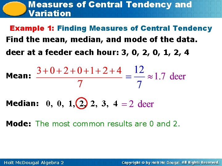
Measures of Central Tendency and Variation Example 1: Finding Measures of Central Tendency Find the mean, median, and mode of the data. deer at a feeder each hour: 3, 0, 2, 0, 1, 2, 4 Mean: Median: 0, 0, 1, 2, 2, 3, 4 Mode: The most common results are 0 and 2. Holt Mc. Dougal Algebra 2

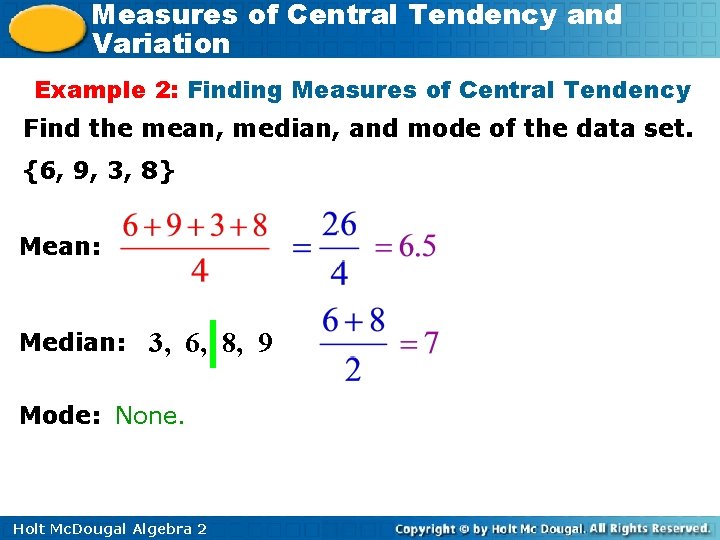
Measures of Central Tendency and Variation Example 2: Finding Measures of Central Tendency Find the mean, median, and mode of the data set. {6, 9, 3, 8} Mean: Median: 3, 6, 8, 9 Mode: None. Holt Mc. Dougal Algebra 2

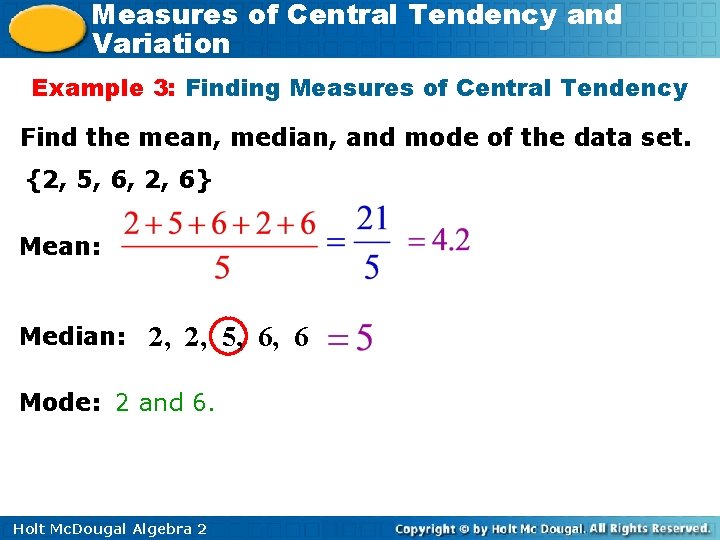
Measures of Central Tendency and Variation Example 3: Finding Measures of Central Tendency Find the mean, median, and mode of the data set. {2, 5, 6, 2, 6} Mean: Median: 2, 2, 5, 6, 6 Mode: 2 and 6. Holt Mc. Dougal Algebra 2

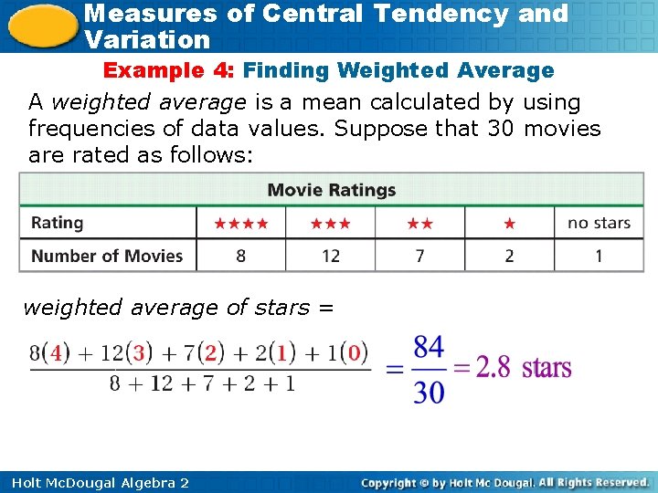
Measures of Central Tendency and Variation Example 4: Finding Weighted Average A weighted average is a mean calculated by using frequencies of data values. Suppose that 30 movies are rated as follows: weighted average of stars = Holt Mc. Dougal Algebra 2

Measures of Central Tendency and Variation For numerical data, the weighted average of all of those outcomes is called the expected value for that experiment. The probability distribution for an experiment is the function that pairs each outcome with its probability. Holt Mc. Dougal Algebra 2

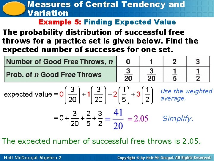
Measures of Central Tendency and Variation Example 5: Finding Expected Value The probability distribution of successful free throws for a practice set is given below. Find the expected number of successes for one set. Use the weighted average. Simplify. The expected number of successful free throws is 2. 05. Holt Mc. Dougal Algebra 2

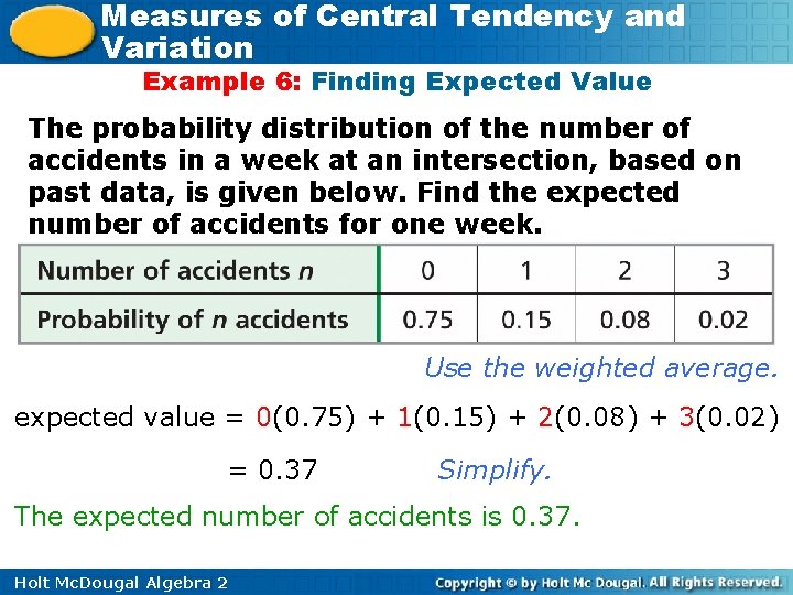
Measures of Central Tendency and Variation Example 6: Finding Expected Value The probability distribution of the number of accidents in a week at an intersection, based on past data, is given below. Find the expected number of accidents for one week. Use the weighted average. expected value = 0(0. 75) + 1(0. 15) + 2(0. 08) + 3(0. 02) = 0. 37 Simplify. The expected number of accidents is 0. 37. Holt Mc. Dougal Algebra 2

Measures of Central Tendency and Variation Lesson 1. 1 Practice A Holt Mc. Dougal Algebra 2

Measures of Central Tendency and Variation • How do we find measures of central tendency and measures of variation for statistical data? • What are the effects of outliers on statistical data? Holt Mc. Dougal Algebra 2

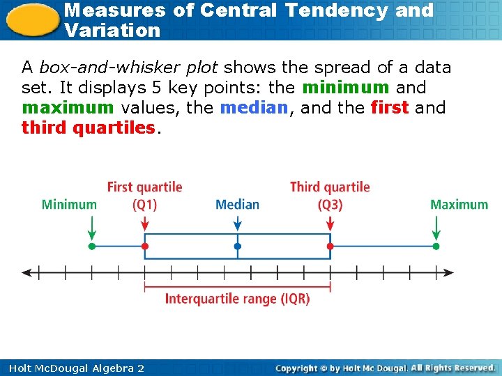
Measures of Central Tendency and Variation A box-and-whisker plot shows the spread of a data set. It displays 5 key points: the minimum and maximum values, the median, and the first and third quartiles. Holt Mc. Dougal Algebra 2

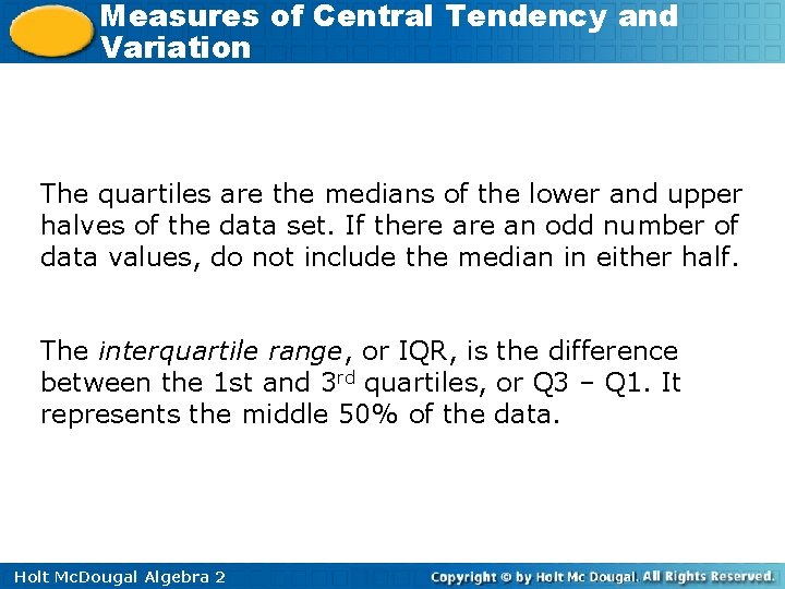
Measures of Central Tendency and Variation The quartiles are the medians of the lower and upper halves of the data set. If there an odd number of data values, do not include the median in either half. The interquartile range, or IQR, is the difference between the 1 st and 3 rd quartiles, or Q 3 – Q 1. It represents the middle 50% of the data. Holt Mc. Dougal Algebra 2

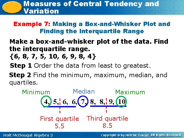
Measures of Central Tendency and Variation Example 7: Making a Box-and-Whisker Plot and Finding the Interquartile Range Make a box-and-whisker plot of the data. Find the interquartile range. {6, 8, 7, 5, 10, 6, 9, 8, 4} Step 1 Order the data from least to greatest. Step 2 Find the minimum, maximum, median, and quartiles. Median Minimum Maximum 4, 5, 6, 6, 7, 8, 8, 9, 10 First quartile 5. 5 Holt Mc. Dougal Algebra 2 Third quartile 8. 5

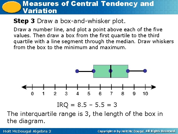
Measures of Central Tendency and Variation Step 3 Draw a box-and-whisker plot. Draw a number line, and plot a point above each of the five values. Then draw a box from the first quartile to the third quartile with a line segment through the median. Draw whiskers from the box to the minimum and maximum. IRQ = 8. 5 – 5. 5 = 3 The interquartile range is 3, the length of the box in the diagram. Holt Mc. Dougal Algebra 2

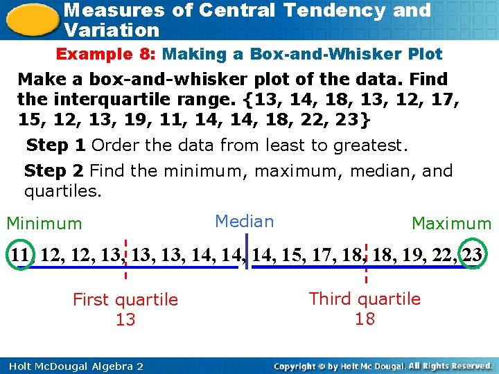
Measures of Central Tendency and Variation Example 8: Making a Box-and-Whisker Plot Make a box-and-whisker plot of the data. Find the interquartile range. {13, 14, 18, 13, 12, 17, 15, 12, 13, 19, 11, 14, 18, 22, 23} Step 1 Order the data from least to greatest. Step 2 Find the minimum, maximum, median, and quartiles. Minimum Median Maximum 11, 12, 13, 13, 14, 14, 15, 17, 18, 19, 22, 23 First quartile 13 Holt Mc. Dougal Algebra 2 Third quartile 18

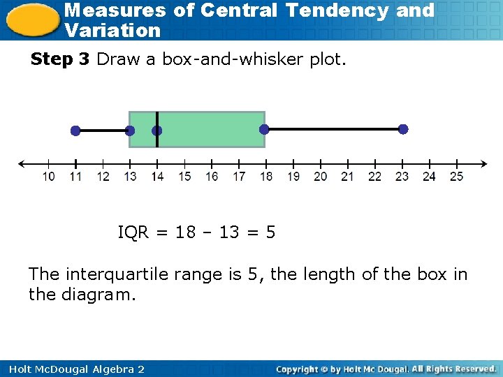
Measures of Central Tendency and Variation Step 3 Draw a box-and-whisker plot. IQR = 18 – 13 = 5 The interquartile range is 5, the length of the box in the diagram. Holt Mc. Dougal Algebra 2

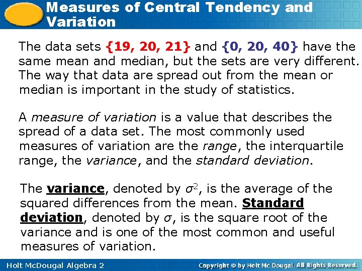
Measures of Central Tendency and Variation The data sets {19, 20, 21} and {0, 20, 40} have the same mean and median, but the sets are very different. The way that data are spread out from the mean or median is important in the study of statistics. A measure of variation is a value that describes the spread of a data set. The most commonly used measures of variation are the range, the interquartile range, the variance, and the standard deviation. The variance, denoted by σ2, is the average of the squared differences from the mean. Standard deviation, denoted by σ, is the square root of the variance and is one of the most common and useful measures of variation. Holt Mc. Dougal Algebra 2

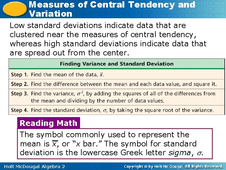
Measures of Central Tendency and Variation Low standard deviations indicate data that are clustered near the measures of central tendency, whereas high standard deviations indicate data that are spread out from the center. Reading Math The symbol commonly used to represent the mean is x, or “x bar. ” The symbol for standard deviation is the lowercase Greek letter sigma, . Holt Mc. Dougal Algebra 2

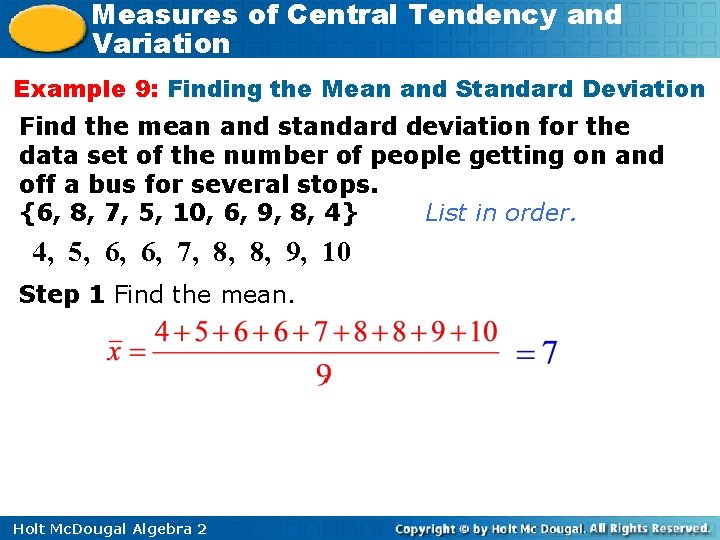
Measures of Central Tendency and Variation Example 9: Finding the Mean and Standard Deviation Find the mean and standard deviation for the data set of the number of people getting on and off a bus for several stops. List in order. {6, 8, 7, 5, 10, 6, 9, 8, 4} 4, 5, 6, 6, 7, 8, 8, 9, 10 Step 1 Find the mean. Holt Mc. Dougal Algebra 2

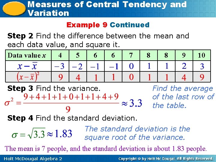
Measures of Central Tendency and Variation Example 9 Continued Step 2 Find the difference between the mean and each data value, and square it. Data value x 4 5 6 6 7 8 8 9 Step 3 Find the variance. 10 Find the average of the last row of the table. Step 4 Find the standard deviation. The standard deviation is the square root of the variance. The mean is 7 people, and the standard deviation is about 1. 83 people. Holt Mc. Dougal Algebra 2

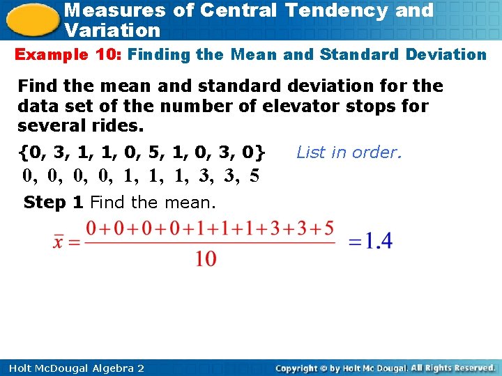
Measures of Central Tendency and Variation Example 10: Finding the Mean and Standard Deviation Find the mean and standard deviation for the data set of the number of elevator stops for several rides. {0, 3, 1, 1, 0, 5, 1, 0, 3, 0} 0, 0, 1, 1, 1, 3, 3, 5 Step 1 Find the mean. Holt Mc. Dougal Algebra 2 List in order.

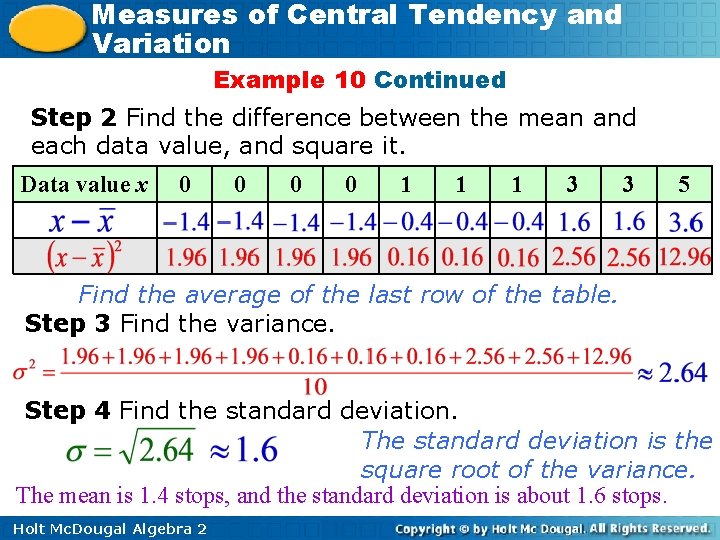
Measures of Central Tendency and Variation Example 10 Continued Step 2 Find the difference between the mean and each data value, and square it. Data value x 0 0 1 1 1 3 3 5 Find the average of the last row of the table. Step 3 Find the variance. Step 4 Find the standard deviation. The standard deviation is the square root of the variance. The mean is 1. 4 stops, and the standard deviation is about 1. 6 stops. Holt Mc. Dougal Algebra 2

Measures of Central Tendency and Variation An outlier is an extreme value that is much less than or much greater than the other data values. Outliers have a strong effect on the mean and standard deviation. If an outlier is the result of measurement error or represents data from the wrong population, it is usually removed. There are different ways to determine whether a value is an outlier. One is to look for data values that are more than 3 standard deviations from the mean. Holt Mc. Dougal Algebra 2

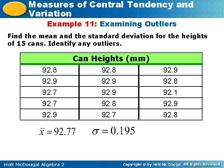
Measures of Central Tendency and Variation Example 11: Examining Outliers Find the mean and the standard deviation for the heights of 15 cans. Identify any outliers. 92. 8 92. 9 92. 7 92. 9 Holt Mc. Dougal Algebra 2 Can Heights (mm) 92. 8 92. 9 92. 8 92. 7 92. 9 92. 8 92. 1 92. 9 92. 8

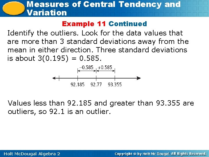
Measures of Central Tendency and Variation Example 11 Continued Identify the outliers. Look for the data values that are more than 3 standard deviations away from the mean in either direction. Three standard deviations is about 3(0. 195) = 0. 585. Values less than 92. 185 and greater than 93. 355 are outliers, so 92. 1 is an outlier. Holt Mc. Dougal Algebra 2

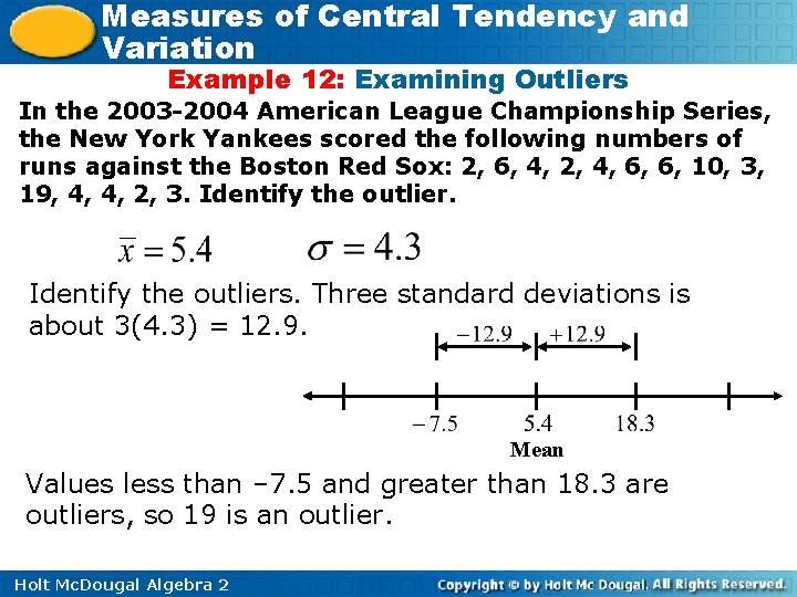
Measures of Central Tendency and Variation Example 12: Examining Outliers In the 2003 -2004 American League Championship Series, the New York Yankees scored the following numbers of runs against the Boston Red Sox: 2, 6, 4, 2, 4, 6, 6, 10, 3, 19, 4, 4, 2, 3. Identify the outliers. Three standard deviations is about 3(4. 3) = 12. 9. Mean Values less than – 7. 5 and greater than 18. 3 are outliers, so 19 is an outlier. Holt Mc. Dougal Algebra 2

Measures of Central Tendency and Variation Lesson 1. 1 Practice B Holt Mc. Dougal Algebra 2