Maximizing the Spread of Influence through a Social

Maximizing the Spread of Influence through a Social Network Authors: David Kempe, Jon Kleinberg, Éva Tardos KDD 2003 Source: 1 http: //www. cs. cmu. edu/~xiaonanz/Maximizing-the-Spread-of-

Social Network and Spread of Influence n Social network plays a fundamental role as a medium for the spread of INFLUENCE among its members q Opinions, ideas, information, innovation… n Direct Marketing takes the “word-ofmouth” effects to significantly increase profits (Gmail, Tupperware popularization, Microsoft Origami …) 2

Problem Setting n Given q q n Goal q n trigger a large cascade of influence (e. g. further adoptions of a product) Question q n a limited budget B for initial advertising (e. g. give away free samples of product) estimates for influence between individuals Which set of individuals should B target at? Application besides product marketing q q spread an innovation detect stories in blogs 3

What we need n n n Form models of influence in social networks. Obtain data about particular network (to estimate inter-personal influence). Devise algorithm to maximize spread of influence. 4

Outline n Models of influence q q n Influence maximization problem q q q n Linear Threshold Independent Cascade Algorithm Proof of performance bound Compute objective function Experiments q q Data and setting Results 5

Outline n Models of influence q q n Influence maximization problem q q q n Linear Threshold Independent Cascade Algorithm Proof of performance bound Compute objective function Experiments q q Data and setting Results 6

Models of Influence n First mathematical models q n Large body of subsequent work: q n n [Schelling '70/'78, Granovetter '78] [Rogers '95, Valente '95, Wasserman/Faust '94] Two basic classes of diffusion models: threshold and cascade General operational view: q q A social network is represented as a directed graph, with each person (customer) as a node Nodes start either active or inactive An active node may trigger activation of neighboring nodes Monotonicity assumption: active nodes never deactivate 7

Outline n Models of influence q q n Influence maximization problem q q q n Linear Threshold Independent Cascade Algorithm Proof of performance bound Compute objective function Experiments q q Data and setting Results 8

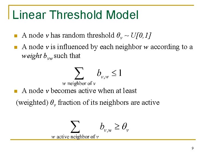
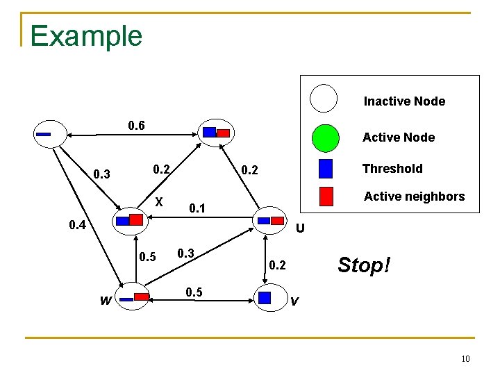
Linear Threshold Model n A node v has random threshold θv ~ U[0, 1] n A node v is influenced by each neighbor w according to a weight bvw such that n A node v becomes active when at least (weighted) θv fraction of its neighbors are active 9

Example Inactive Node 0. 6 0. 3 Active Node 0. 2 X Threshold 0. 2 Active neighbors 0. 1 0. 4 U 0. 5 w 0. 3 0. 5 Stop! 0. 2 v 10

Outline n Models of influence q q n Influence maximization problem q q q n Linear Threshold Independent Cascade Algorithm Proof of performance bound Compute objective function Experiments q q Data and setting Results 11

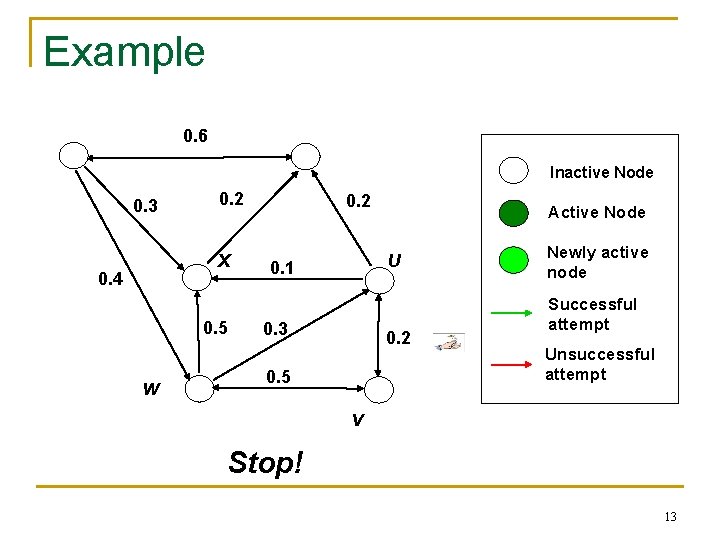
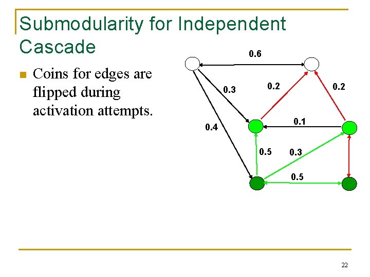
Independent Cascade Model n n When node v becomes active, it has a single chance of activating each currently inactive neighbor w. The activation attempt succeeds with probability pvw. 12

Example 0. 6 Inactive Node 0. 3 0. 2 X 0. 4 0. 5 w 0. 2 Active Node U 0. 1 0. 3 0. 2 0. 5 Newly active node Successful attempt Unsuccessful attempt v Stop! 13

Outline n Models of influence q q n Influence maximization problem q q q n Linear Threshold Independent Cascade Algorithm Proof of performance bound Compute objective function Experiments q q Data and setting Results 14

Influence Maximization Problem n Influence of node set S: f(S) q n expected number of active nodes at the end, if set S is the initial active set Problem: q q Given a parameter k (budget), find a k-node set S to maximize f(S) Constrained optimization problem with f(S) as the objective function 15

Outline n Models of influence q q n Influence maximization problem q q q n Linear Threshold Independent Cascade Algorithm Proof of performance bound Compute objective function Experiments q q Data and setting Results 16

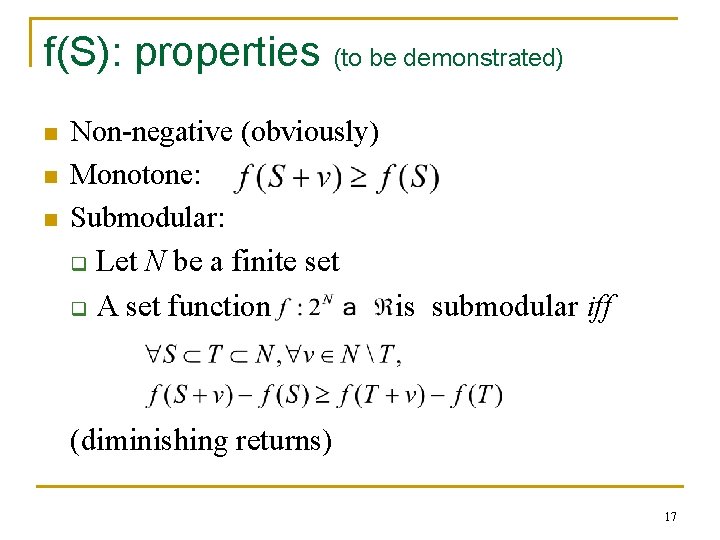
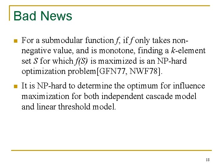
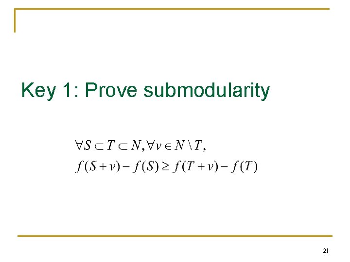
f(S): properties (to be demonstrated) n n n Non-negative (obviously) Monotone: Submodular: q Let N be a finite set q A set function is submodular iff (diminishing returns) 17

Bad News n For a submodular function f, if f only takes nonnegative value, and is monotone, finding a k-element set S for which f(S) is maximized is an NP-hard optimization problem[GFN 77, NWF 78]. n It is NP-hard to determine the optimum for influence maximization for both independent cascade model and linear threshold model. 18

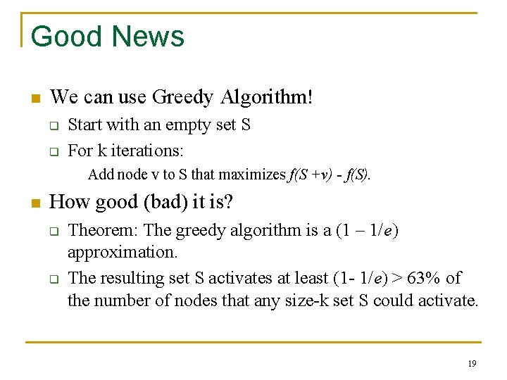
Good News n We can use Greedy Algorithm! q q Start with an empty set S For k iterations: Add node v to S that maximizes f(S +v) - f(S). n How good (bad) it is? q q Theorem: The greedy algorithm is a (1 – 1/e) approximation. The resulting set S activates at least (1 - 1/e) > 63% of the number of nodes that any size-k set S could activate. 19

Outline n Models of influence q q n Influence maximization problem q q q n Linear Threshold Independent Cascade Algorithm Proof of performance bound Compute objective function Experiments q q Data and setting Results 20

Key 1: Prove submodularity 21

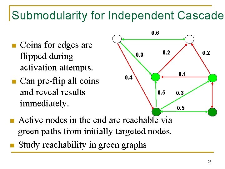
Submodularity for Independent Cascade 0. 6 n Coins for edges are flipped during activation attempts. 0. 3 0. 2 0. 1 0. 4 0. 5 0. 3 0. 5 22

Submodularity for Independent Cascade 0. 6 n n Coins for edges are flipped during activation attempts. Can pre-flip all coins and reveal results immediately. 0. 3 0. 2 0. 1 0. 4 0. 5 0. 3 0. 5 Active nodes in the end are reachable via green paths from initially targeted nodes. Study reachability in green graphs 23

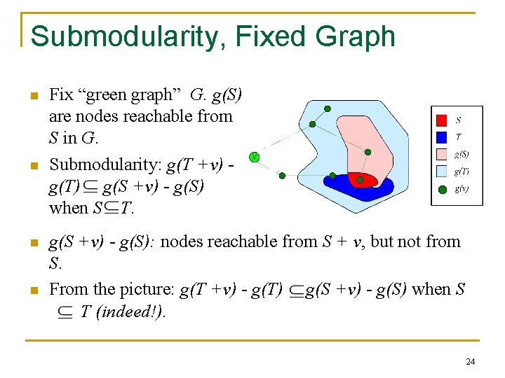
Submodularity, Fixed Graph n n Fix “green graph” G. g(S) are nodes reachable from S in G. Submodularity: g(T +v) g(T) g(S +v) - g(S) when S T. g(S +v) - g(S): nodes reachable from S + v, but not from S. From the picture: g(T +v) - g(T) g(S +v) - g(S) when S T (indeed!). 24

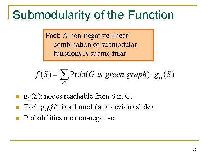
Submodularity of the Function Fact: A non-negative linear combination of submodular functions is submodular n n n g. G(S): nodes reachable from S in G. Each g. G(S): is submodular (previous slide). Probabilities are non-negative. 25

Submodularity for Linear Threshold n n n Use similar “green graph” idea. Once a graph is fixed, “reachability” argument is identical. How do we fix a green graph now? Assume every time nodes pick their threshold uniformly from [0 -1]. Each node picks at most one incoming edge, with probabilities proportional to edge weights. Equivalent to linear threshold model (trickier proof). 26

Outline n Models of influence q q n Influence maximization problem q q q n Linear Threshold Independent Cascade Algorithm Proof of performance bound Compute objective function Experiments q q Data and setting Results 27

Key 2: Evaluating f(S) 28

Evaluating ƒ(S) n n n How to evaluate ƒ(S)? Still an open question of how to compute efficiently But: very good estimates by simulation q q n Generate green graph G’ often enough (polynomial in n; 1/ε). Apply Greedy algorithm to G’. Achieve (1± ε)-approximation to f(S). Generalization of Nemhauser/Wolsey proof shows: Greedy algorithm is now a (1 -1/e- ε′)approximation. 29

Outline n Models of influence q q n Influence maximization problem q q q n Linear Threshold Independent Cascade Algorithm Proof of performance bound Compute objective function Experiments q q Data and setting Results 30

Experiment Data n n n A collaboration graph obtained from coauthorships in papers of the ar. Xiv high-energy physics theory section co-authorship networks arguably capture many of the key features of social networks more generally Resulting graph: 10748 nodes, 53000 distinct edges 31

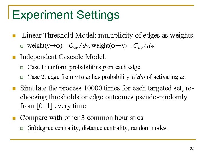
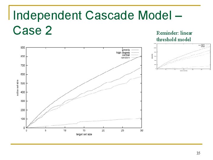
Experiment Settings n Linear Threshold Model: multiplicity of edges as weights q n weight(v→ω) = Cvw / dv, weight(ω→v) = Cwv / dw Independent Cascade Model: q Case 1: uniform probabilities p on each edge q Case 2: edge from v to ω has probability 1/ dω of activating ω. n Simulate the process 10000 times for each targeted set, rechoosing thresholds or edge outcomes pseudo-randomly from [0, 1] every time n Compare with other 3 common heuristics q (in)degree centrality, distance centrality, random nodes. 32

Outline n Models of influence q q n Influence maximization problem q q q n Linear Threshold Independent Cascade Algorithm Proof of performance bound Compute objective function Experiments q q Data and setting Results 33

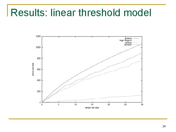
Results: linear threshold model 34

Independent Cascade Model – Case 2 Reminder: linear threshold model 35

More in the Paper n n n A broader framework that simultaneously generalizes the two models Non-progressive process: active nodes CAN deactivate. More realistic marketing: different marketing actions increase likelihood of initial activation, for several nodes at once. q 36

Open Questions n n Study more general influence models. Find trade-offs between generality and feasibility. Deal with negative influences. Model competing ideas. Obtain more data about how activations occur in real social networks. 37

Thanks! 38

Influence Maximization When Negative Opinions may Emerge and Propagate Authors: Wei Chan and lot others Microsoft Research Technical Report 2010 39

Outline n n n Model of influence f(S) Sub-modular Other models 40

Model of Influence n Similar to independent cascade model. q q n n n When node v becomes active, it has a single chance of activating each currently inactive neighbor w. The activation attempt succeeds with probability pvw. If node v is negative then node w also becomes negative. If node v is positive then node w becomes positive with probability q else becomes negative. q is the product quality factor. 41

Model of Influence n Intuition: q q q Negative opinions originate from imperfect product/service quality. Negative node generates the negative opinions. Positive and Negative opinions are asymmetric n Negative opinions are generally much stronger. 42

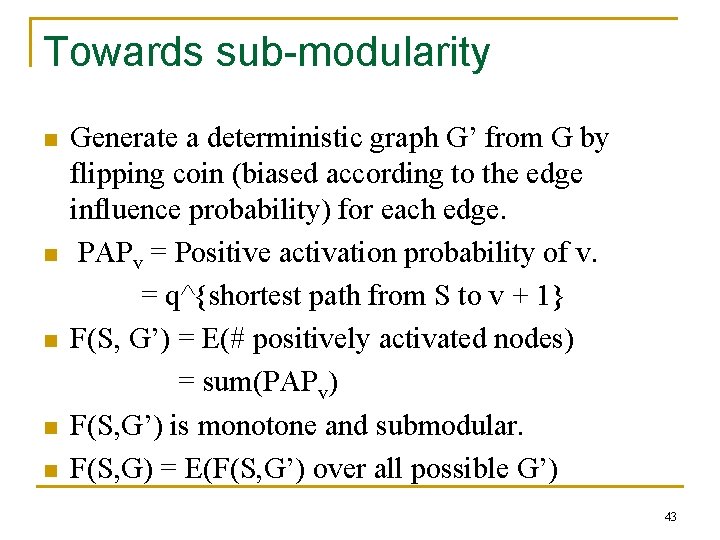
Towards sub-modularity n n n Generate a deterministic graph G’ from G by flipping coin (biased according to the edge influence probability) for each edge. PAPv = Positive activation probability of v. = q^{shortest path from S to v + 1} F(S, G’) = E(# positively activated nodes) = sum(PAPv) F(S, G’) is monotone and submodular. F(S, G) = E(F(S, G’) over all possible G’) 43

Other models n n n Different quality factor for every node Stronger negative influence probability Different propagation delays None of them are sub-modular in nature! 44