macro Money and Inflation U S inflation and

macro Money and Inflation

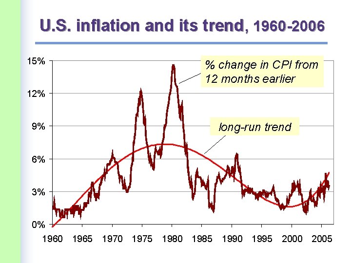
U. S. inflation and its trend, 1960 -2006 15% % change in CPI from 12 months earlier 12% long-run trend 9% 6% 3% 0% 1960 1965 1970 1975 1980 1985 1990 1995 2000 2005

Money: Functions § medium of exchange § store of value § unit of account

Money: Types 1. fiat money – has no intrinsic value – example: the paper currency we use 2. commodity money – has intrinsic value – examples: gold coins, cigarettes in P. O. W. camps

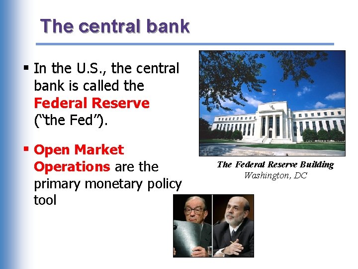
The central bank § In the U. S. , the central bank is called the Federal Reserve (“the Fed”). § Open Market Operations are the primary monetary policy tool The Federal Reserve Building Washington, DC

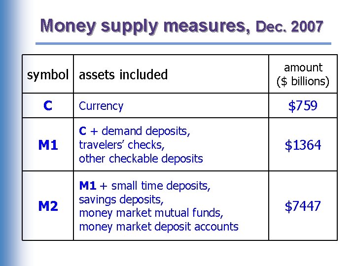
Money supply measures, Dec. 2007 symbol assets included C Currency amount ($ billions) $759 M 1 C + demand deposits, travelers’ checks, other checkable deposits $1364 M 2 M 1 + small time deposits, savings deposits, money market mutual funds, money market deposit accounts $7447

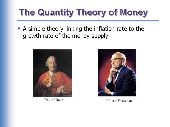
The Quantity Theory of Money § A simple theory linking the inflation rate to the growth rate of the money supply. David Hume Milton Friedman

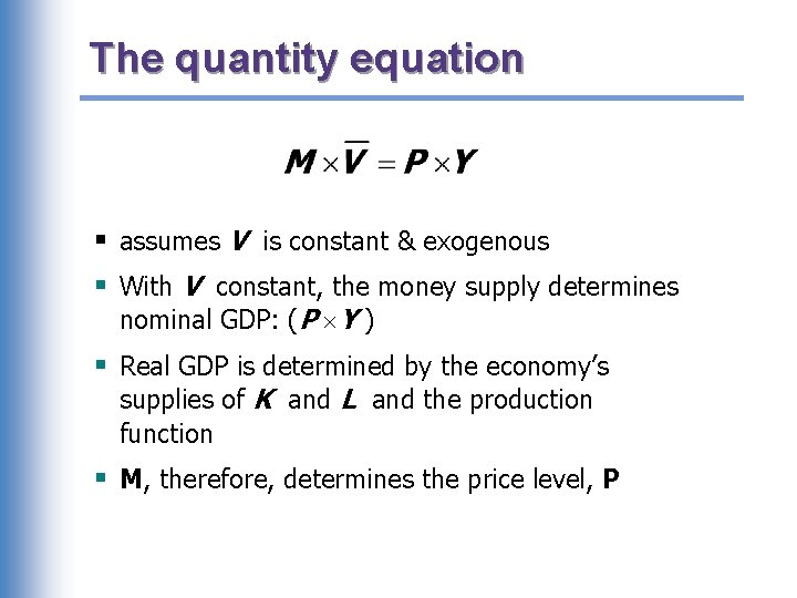
The quantity equation § assumes V is constant & exogenous § With V constant, the money supply determines nominal GDP: (P Y ) § Real GDP is determined by the economy’s supplies of K and L and the production function § M, therefore, determines the price level, P

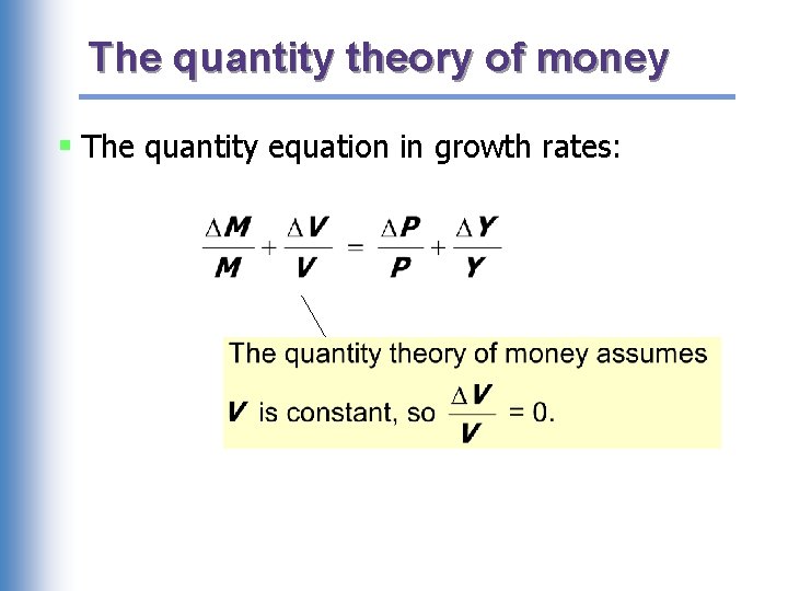
The quantity theory of money § The quantity equation in growth rates:

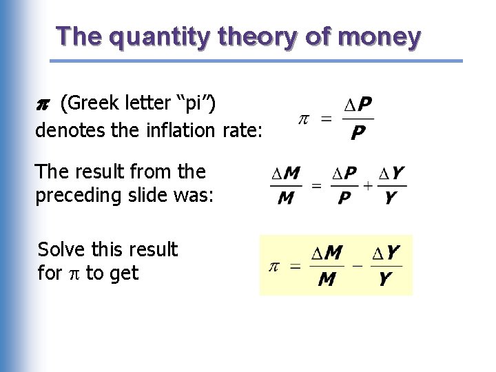
The quantity theory of money (Greek letter “pi”) denotes the inflation rate: The result from the preceding slide was: Solve this result for to get

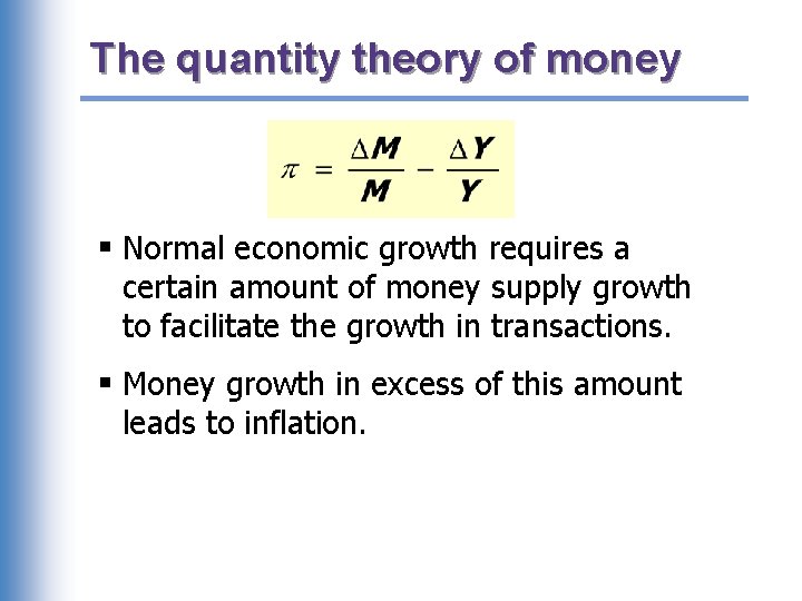
The quantity theory of money § Normal economic growth requires a certain amount of money supply growth to facilitate the growth in transactions. § Money growth in excess of this amount leads to inflation.

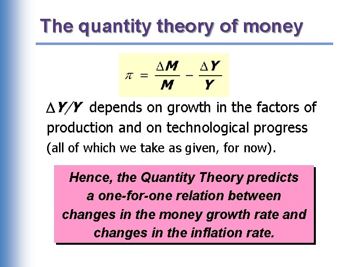
The quantity theory of money Y/Y depends on growth in the factors of production and on technological progress (all of which we take as given, for now). Hence, the Quantity Theory predicts a one-for-one relation between changes in the money growth rate and changes in the inflation rate.

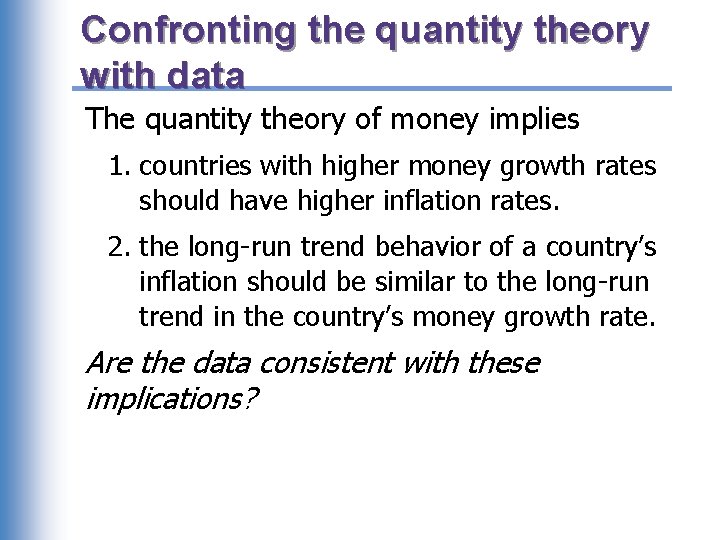
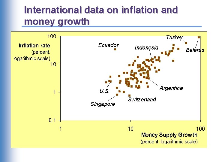
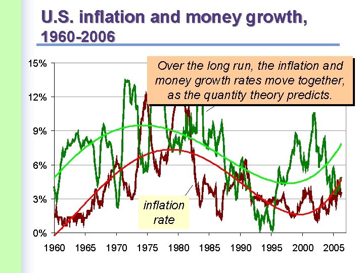
Confronting the quantity theory with data The quantity theory of money implies 1. countries with higher money growth rates should have higher inflation rates. 2. the long-run trend behavior of a country’s inflation should be similar to the long-run trend in the country’s money growth rate. Are the data consistent with these implications?

International data on inflation and money growth Turkey Ecuador Indonesia Argentina U. S. Singapore Belarus Switzerland

U. S. inflation and money growth, 1960 -2006 15% 12% Over the long run, the inflation and money growth rates move together, M 2 growth as the quantity theory rate predicts. 9% 6% 3% 0% 1960 1965 inflation rate 1970 1975 1980 1985 1990 1995 2000 2005

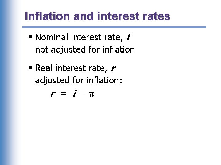
Inflation and interest rates § Nominal interest rate, i not adjusted for inflation § Real interest rate, r adjusted for inflation: r = i

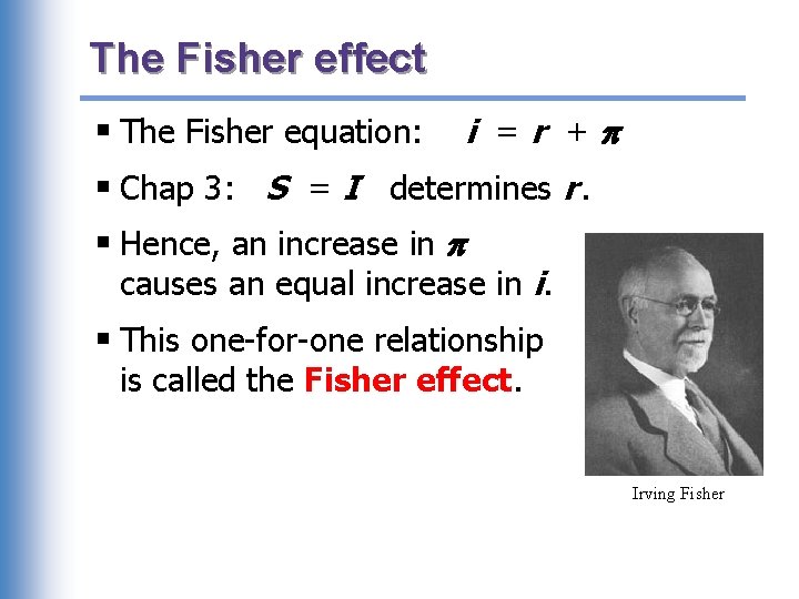
The Fisher effect § The Fisher equation: i =r + § Chap 3: S = I determines r. § Hence, an increase in causes an equal increase in i. § This one-for-one relationship is called the Fisher effect. Irving Fisher

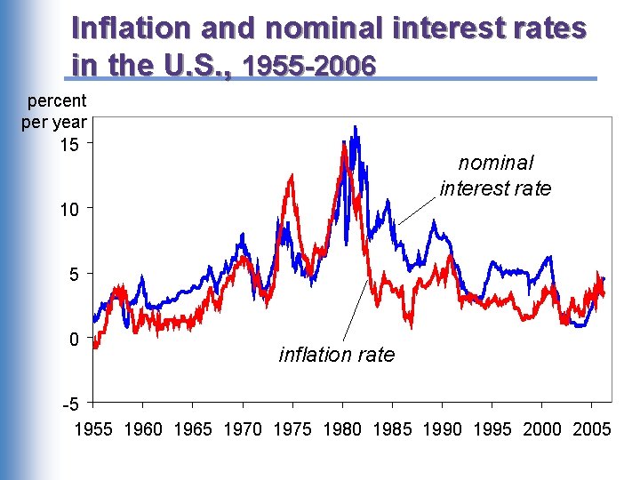
Inflation and nominal interest rates in the U. S. , 1955 -2006 percent per year 15 nominal interest rate 10 5 0 inflation rate -5 1955 1960 1965 1970 1975 1980 1985 1990 1995 2000 2005

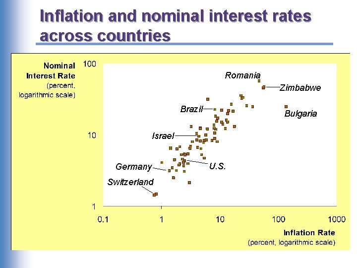
Inflation and nominal interest rates across countries Romania Zimbabwe Brazil Bulgaria Israel Germany Switzerland U. S.

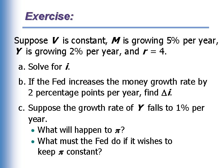
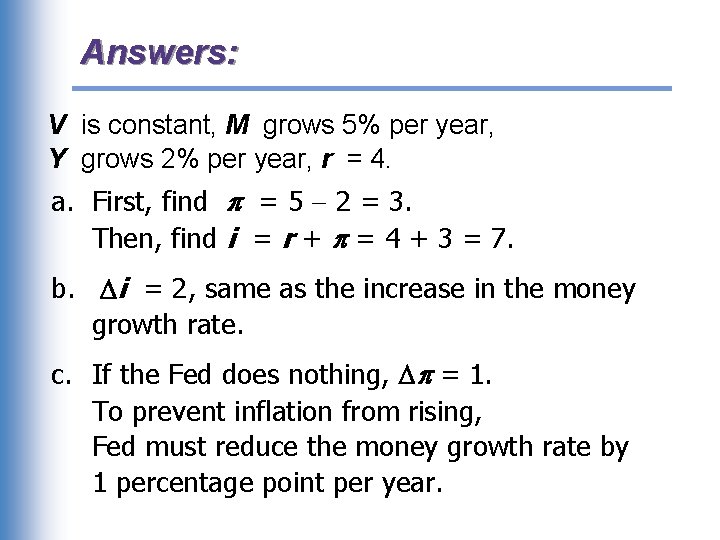
Exercise: Suppose V is constant, M is growing 5% per year, Y is growing 2% per year, and r = 4. a. Solve for i. b. If the Fed increases the money growth rate by 2 percentage points per year, find i. c. Suppose the growth rate of Y falls to 1% per year. • What will happen to ? • What must the Fed do if it wishes to keep constant?

Answers: V is constant, M grows 5% per year, Y grows 2% per year, r = 4. a. First, find = 5 2 = 3. Then, find i = r + = 4 + 3 = 7. b. i = 2, same as the increase in the money growth rate. c. If the Fed does nothing, = 1. To prevent inflation from rising, Fed must reduce the money growth rate by 1 percentage point per year.

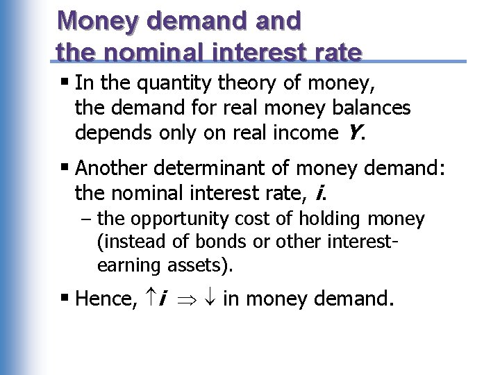
Money demand the nominal interest rate § In the quantity theory of money, the demand for real money balances depends only on real income Y. § Another determinant of money demand: the nominal interest rate, i. – the opportunity cost of holding money (instead of bonds or other interestearning assets). § Hence, i in money demand.

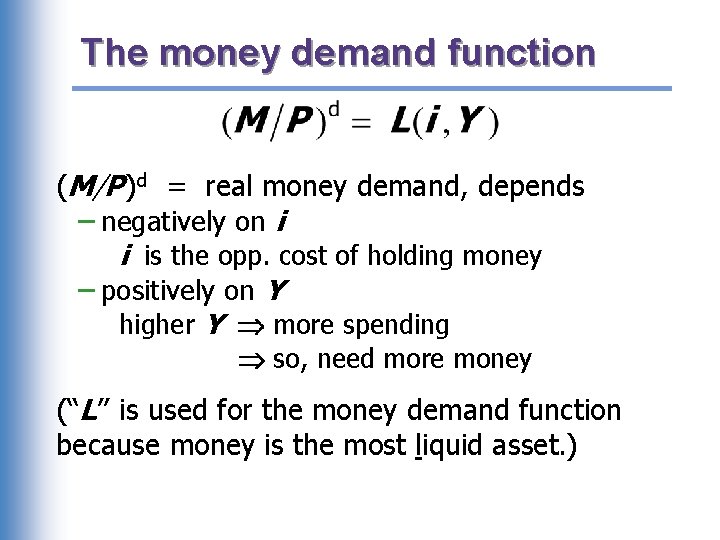
The money demand function (M/P )d = real money demand, depends – negatively on i i is the opp. cost of holding money – positively on Y higher Y more spending so, need more money (“L” is used for the money demand function because money is the most liquid asset. )

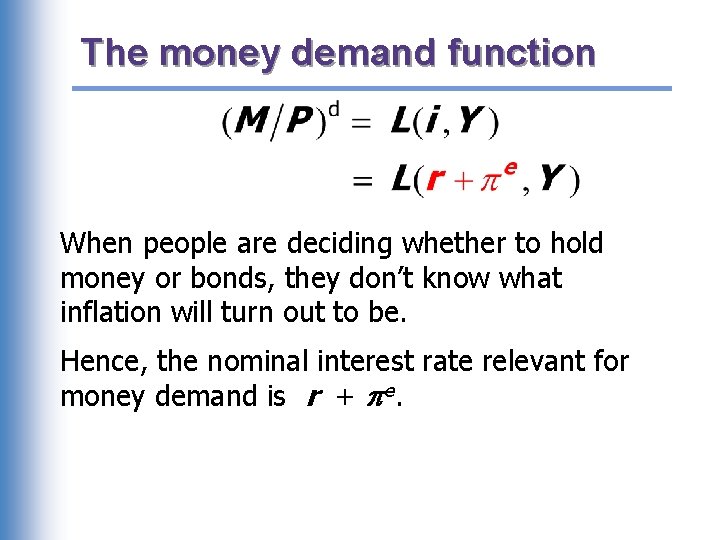
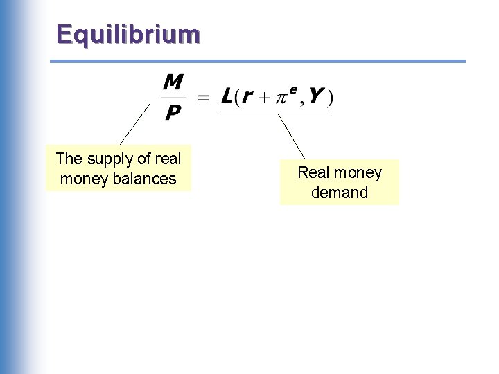
The money demand function When people are deciding whether to hold money or bonds, they don’t know what inflation will turn out to be. Hence, the nominal interest rate relevant for money demand is r + e.

Equilibrium The supply of real money balances Real money demand

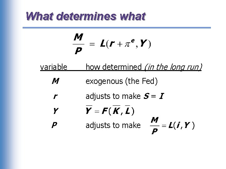
What determines what variable how determined (in the long run) M exogenous (the Fed) r adjusts to make S = I Y P adjusts to make

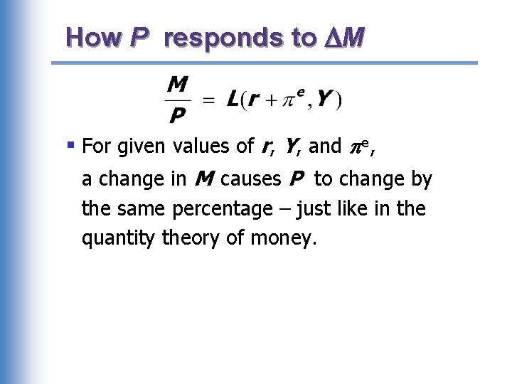
How P responds to M § For given values of r, Y, and e, a change in M causes P to change by the same percentage – just like in the quantity theory of money.

Discussion question Why is inflation bad? § What costs does inflation impose on society? List all the ones you can think of. § Focus on the long run.

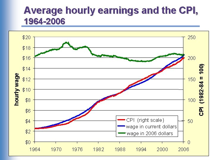
A common misperception § Common misperception: inflation reduces real wages § This is true only in the short run, when nominal wages are fixed by contracts. § (Chap. 3) In the long run, the real wage is determined by labor supply and the marginal product of labor, not the price level or inflation rate. § Consider the data…

Average hourly earnings and the CPI, 1964 -2006 $20 250 $18 200 hourly wage $14 $12 150 $10 $8 100 $6 CPI (right scale) wage in current dollars wage in 2006 dollars $4 $2 $0 1964 1970 1976 1982 1988 1994 2000 50 0 2006 CPI (1982 -84 = 100) $16

The classical view of inflation § The classical view: A change in the price level is merely a change in the units of measurement. So why, then, is inflation a social problem?

The social costs of inflation …fall into two categories: 1. costs when inflation is expected 2. costs when inflation is different than people had expected

The costs of expected inflation: § Shoeleather cost § Menu costs § Relative price distortions § Unfair tax treatment § General inconvenience

The cost of unexpected inflation: § Arbitrary redistribution of purchasing power – Ex: From lenders to borrowers § Increased uncertainty

One benefit of inflation § Nominal wages are rarely reduced, even when the equilibrium real wage falls. This hinders labor market clearing. § Inflation allows the real wages to reach equilibrium levels without nominal wage cuts. § Therefore, moderate inflation improves the functioning of labor markets.

Hyperinflation § def: 50% per month § All the costs of moderate inflation described above become HUGE under hyperinflation. § Money ceases to function as a store of value, and may not serve its other functions (unit of account, medium of exchange). § People may conduct transactions with barter or a stable foreign currency.

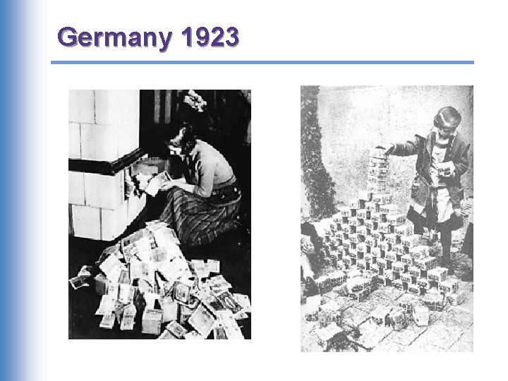
Germany 1923

What causes hyperinflation? § Hyperinflation is caused by excessive money supply growth: § When the central bank prints money, the price level rises. § If it prints money rapidly enough, the result is hyperinflation.

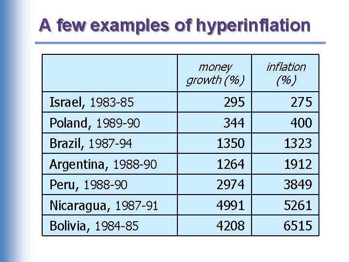
A few examples of hyperinflation money growth (%) inflation (%) Israel, 1983 -85 295 275 Poland, 1989 -90 344 400 Brazil, 1987 -94 1350 1323 Argentina, 1988 -90 1264 1912 Peru, 1988 -90 2974 3849 Nicaragua, 1987 -91 4991 5261 Bolivia, 1984 -85 4208 6515

Why governments create hyperinflation § When a government cannot raise taxes or sell bonds, § it must finance spending increases by printing money. § In theory, the solution to hyperinflation is simple: stop printing money. § In the real world, this requires drastic and painful fiscal restraint.

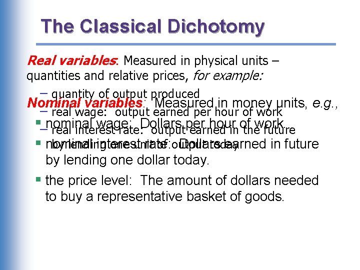
The Classical Dichotomy Real variables: Measured in physical units – quantities and relative prices, for example: – quantity of output produced Nominal variables: Measured in money units, e. g. , – real wage: output earned per hour of work §–nominal wage: Dollars per hour of work. real interest rate: output earned in the future § nominal interest rate: Dollars earned in future by lending one unit of output today by lending one dollar today. § the price level: The amount of dollars needed to buy a representative basket of goods.

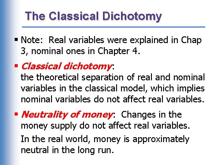
The Classical Dichotomy § Note: Real variables were explained in Chap 3, nominal ones in Chapter 4. § Classical dichotomy: theoretical separation of real and nominal variables in the classical model, which implies nominal variables do not affect real variables. § Neutrality of money: Changes in the money supply do not affect real variables. In the real world, money is approximately neutral in the long run.

macro Unemployment

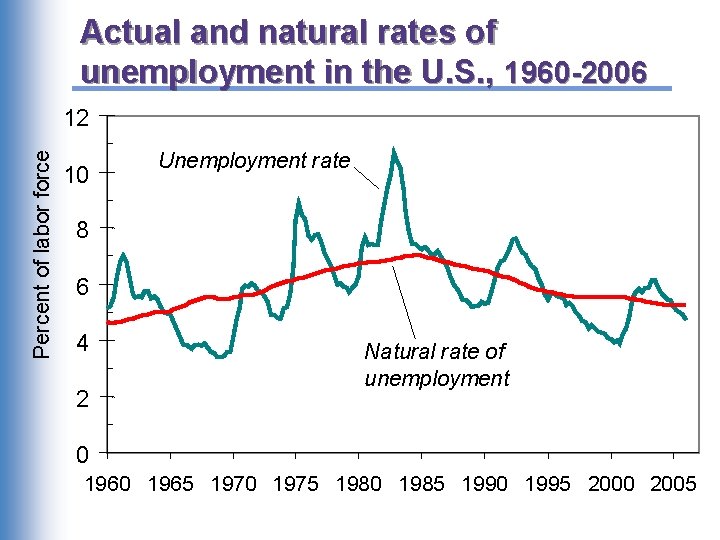
Actual and natural rates of unemployment in the U. S. , 1960 -2006 Percent of labor force 12 10 Unemployment rate 8 6 4 2 Natural rate of unemployment 0 1965 1970 1975 1980 1985 1990 1995 2000 2005

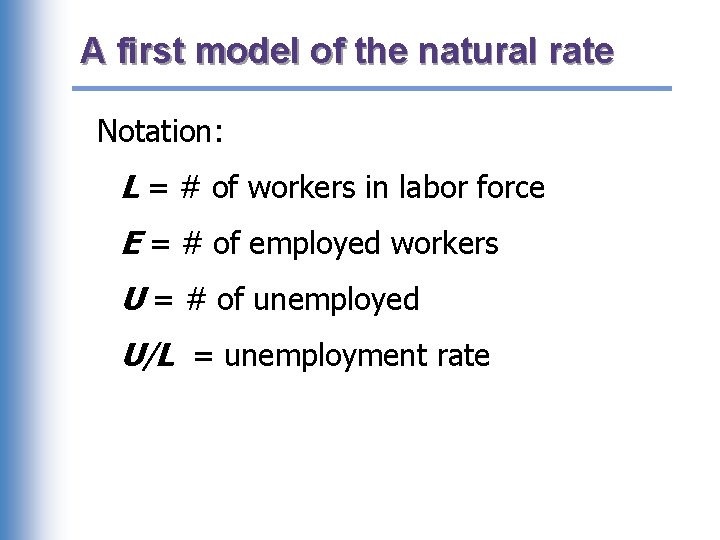
A first model of the natural rate Notation: L = # of workers in labor force E = # of employed workers U = # of unemployed U/L = unemployment rate

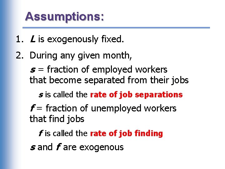
Assumptions: 1. L is exogenously fixed. 2. During any given month, s = fraction of employed workers that become separated from their jobs s is called the rate of job separations f = fraction of unemployed workers that find jobs f is called the rate of job finding s and f are exogenous

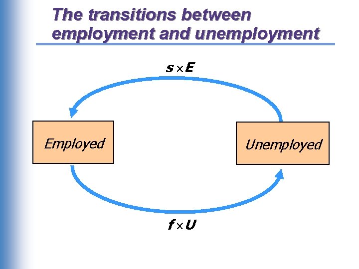
The transitions between employment and unemployment s E Employed Unemployed f U

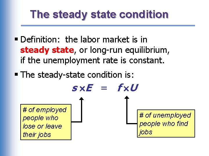
The steady state condition § Definition: the labor market is in steady state, or long-run equilibrium, if the unemployment rate is constant. § The steady-state condition is: s E = f U # of employed people who lose or leave their jobs # of unemployed people who find jobs

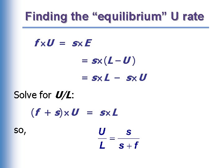
Finding the “equilibrium” U rate f U = s E = s (L – U ) = s L – s U Solve for U/L: (f + s) U = s L so,

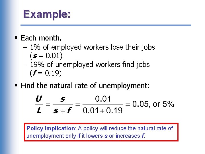
Example: § Each month, – 1% of employed workers lose their jobs (s = 0. 01) – 19% of unemployed workers find jobs (f = 0. 19) § Find the natural rate of unemployment: Policy Implication: A policy will reduce the natural rate of unemployment only if it lowers s or increases f.

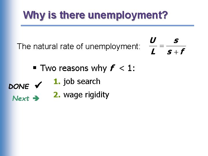
Why is there unemployment? § If job finding were instantaneous (f = 1), then all spells of unemployment would be brief, and the natural rate would be near zero. § There are two reasons why f < 1: 1. job search 2. wage rigidity

Job search & frictional unemployment § frictional unemployment: caused by the time it takes workers to search for a job § occurs even when wages are flexible and there are enough jobs to go around § occurs because – – workers have different abilities, preferences jobs have different skill requirements geographic mobility of workers not instantaneous flow of information about vacancies and job candidates is imperfect

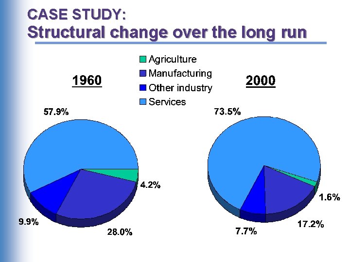
Sectoral shifts § def: Changes in the composition of demand among industries or regions. § example: Technological change more jobs repairing computers, fewer jobs repairing typewriters § example: A new international trade agreement labor demand increases in export sectors, decreases in import-competing sectors § Result: frictional unemployment

CASE STUDY: Structural change over the long run

Public policy and job search Govt programs affecting unemployment – Govt employment agencies: disseminate info about job openings to better match workers & jobs. – Public job training programs: help workers displaced from declining industries get skills needed for jobs in growing industries.

Unemployment insurance (UI) § UI pays part of a worker’s former wages for a limited time after losing his/her job. § UI increases search unemployment, because it reduces – the opportunity cost of being unemployed – the urgency of finding work –f § Studies: The longer a worker is eligible for UI, the longer the duration of the average spell of unemployment.

Benefits of UI § By allowing workers more time to search, UI may lead to better matches between jobs and workers, which would lead to greater productivity and higher incomes.

Why is there unemployment? The natural rate of unemployment: § Two reasons why f < 1: DONE Next 1. job search 2. wage rigidity

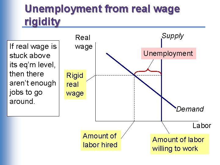
Unemployment from real wage rigidity If real wage is stuck above its eq’m level, then there aren’t enough jobs to go around. Real wage Supply Unemployment Rigid real wage Demand Labor Amount of labor hired Amount of labor willing to work

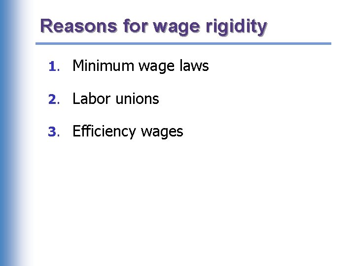
Reasons for wage rigidity 1. Minimum wage laws 2. Labor unions 3. Efficiency wages

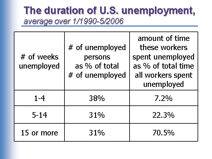
The duration of U. S. unemployment, average over 1/1990 -5/2006 # of weeks unemployed amount of time # of unemployed these workers persons spent unemployed as % of total time # of unemployed all workers spent unemployed 1 -4 38% 7. 2% 5 -14 31% 22. 3% 15 or more 31% 70. 5%

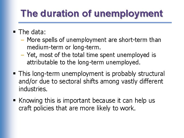
The duration of unemployment § The data: – More spells of unemployment are short-term than medium-term or long-term. – Yet, most of the total time spent unemployed is attributable to the long-term unemployed. § This long-term unemployment is probably structural and/or due to sectoral shifts among vastly different industries. § Knowing this is important because it can help us craft policies that are more likely to work.

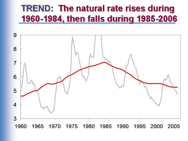
TREND: The natural rate rises during 1960 -1984, then falls during 1985 -2006

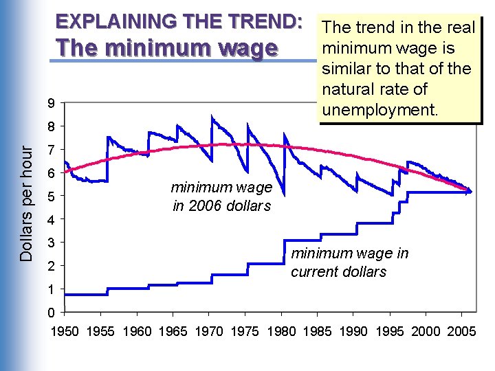
EXPLAINING THE TREND: The trend in the real The minimum wage 9 minimum wage is similar to that of the natural rate of unemployment. Dollars per hour 8 7 6 5 4 3 2 minimum wage in 2006 dollars minimum wage in current dollars 1 0 1955 1960 1965 1970 1975 1980 1985 1990 1995 2000 2005

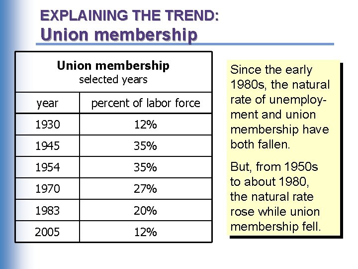
EXPLAINING THE TREND: Union membership selected years year percent of labor force 1930 12% 1945 35% 1954 35% 1970 27% 1983 20% 2005 12% Since the early 1980 s, the natural rate of unemployment and union membership have both fallen. But, from 1950 s to about 1980, the natural rate rose while union membership fell.

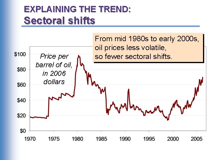
EXPLAINING THE TREND: Sectoral shifts Price per barrel of oil, in 2006 dollars From mid 1980 s to early 2000 s, oil prices less volatile, so fewer sectoral shifts.

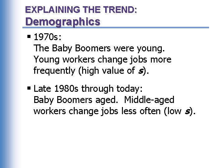
EXPLAINING THE TREND: Demographics § 1970 s: The Baby Boomers were young. Young workers change jobs more frequently (high value of s). § Late 1980 s through today: Baby Boomers aged. Middle-aged workers change jobs less often (low s).

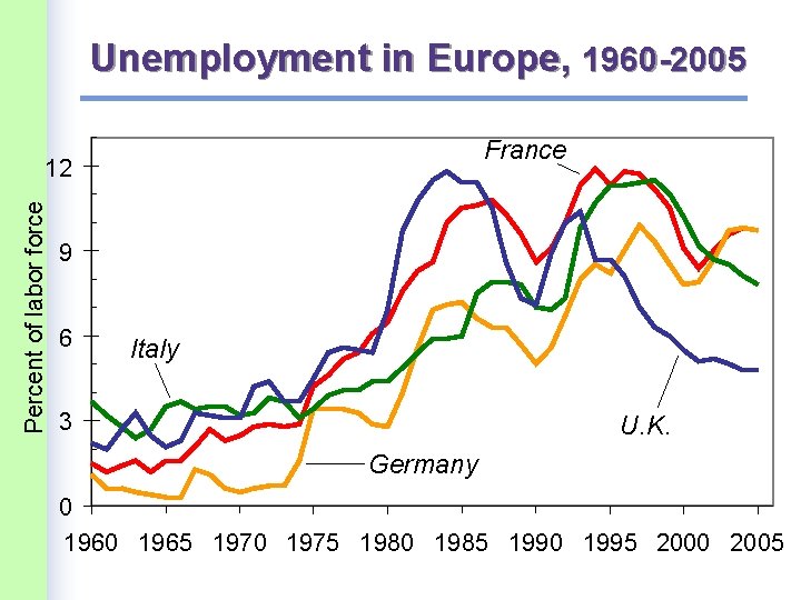
Unemployment in Europe, 1960 -2005 France Percent of labor force 12 9 6 Italy 3 U. K. Germany 0 1965 1970 1975 1980 1985 1990 1995 2000 2005

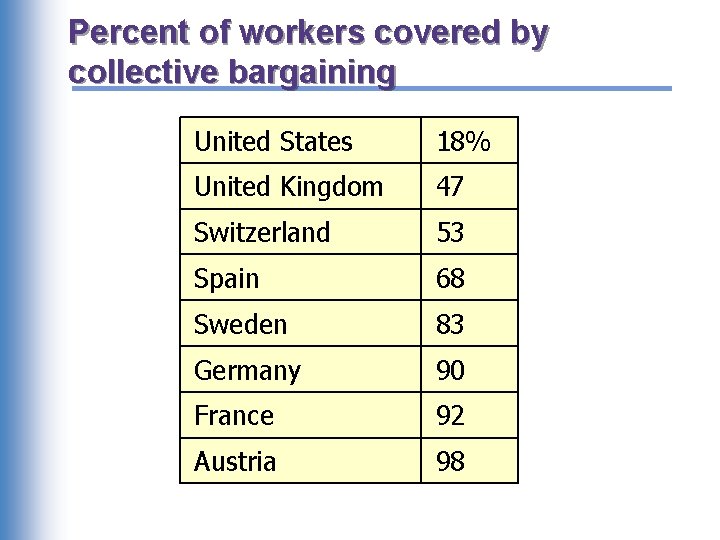
The rise in European unemployment § Shock Technological progress has shifted labor demand from unskilled to skilled workers in recent decades. § Effect in United States An increase in the “skill premium” – the wage gap between skilled and unskilled workers. § Effect in Europe Higher unemployment, due to generous govt benefits for unemployed workers and strong union presence.

Percent of workers covered by collective bargaining United States 18% United Kingdom 47 Switzerland 53 Spain 68 Sweden 83 Germany 90 France 92 Austria 98