Linear Filtering Part I Selim Aksoy Department of

Linear Filtering – Part I Selim Aksoy Department of Computer Engineering Bilkent University saksoy@cs. bilkent. edu. tr

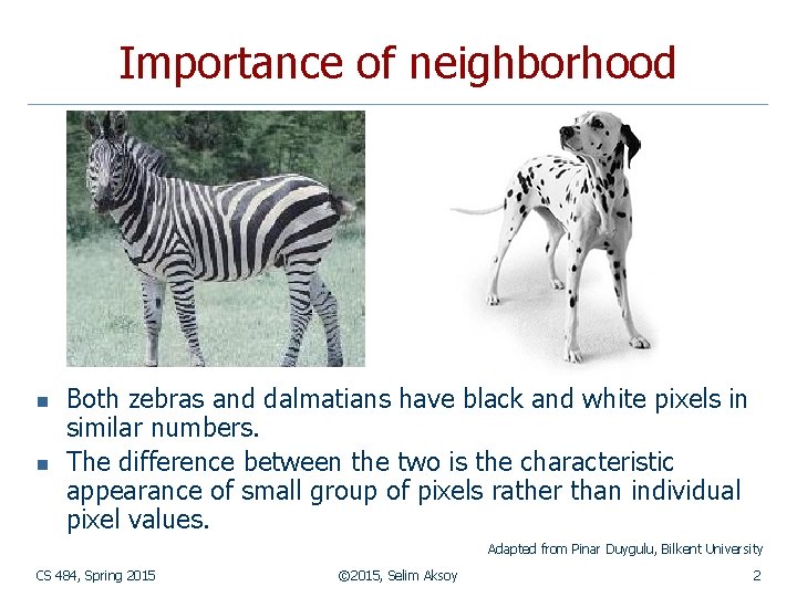
Importance of neighborhood n n Both zebras and dalmatians have black and white pixels in similar numbers. The difference between the two is the characteristic appearance of small group of pixels rather than individual pixel values. Adapted from Pinar Duygulu, Bilkent University CS 484, Spring 2015 © 2015, Selim Aksoy 2

Outline n n n We will discuss neighborhood operations that work with the values of the image pixels in the neighborhood. Spatial domain filtering Frequency domain filtering Image enhancement Finding patterns CS 484, Spring 2015 © 2015, Selim Aksoy 3

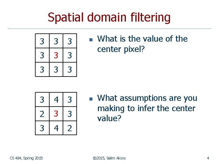
Spatial domain filtering 3 3 3 ? 3 3 3 4 3 2 3 ? 3 3 4 2 CS 484, Spring 2015 n n What is the value of the center pixel? What assumptions are you making to infer the center value? © 2015, Selim Aksoy 4

Spatial domain filtering n Some neighborhood operations work with n n the values of the image pixels in the neighborhood, and the corresponding values of a subimage that has the same dimensions as the neighborhood. The subimage is called a filter (or mask, kernel, template, window). The values in a filter subimage are referred to as coefficients, rather than pixels. CS 484, Spring 2015 © 2015, Selim Aksoy 5

Spatial domain filtering n n n Operation: modify the pixels in an image based on some function of the pixels in their neighborhood. Simplest: linear filtering (replace each pixel by a linear combination of its neighbors). Linear spatial filtering is often referred to as “convolving an image with a filter”. CS 484, Spring 2015 © 2015, Selim Aksoy 6

Linear filtering Linear system: 2 Input: h [m] 0 Output? -1 1 2 g [m] 2 2 2 1 0 2 -1 h [-k] h [1 -k] 1 0 1 -1 -1 2 2 2 1 1 0 3 f [m=0]=-2 f [m=1]=-4 0 -1 1 2 -1 f [m=2]=0 CS 484, Spring 2015 © 2015, Selim Aksoy 7

Linear filtering g [m, n] f [m, n] For a linear spatially invariant system m=0 1 2 … 111 115 113 111 112 111 ? ? 135 138 137 139 145 146 149 147 ? -5 9 -9 21 -12 10 ? 163 168 188 196 202 206 207 ? -29 18 24 4 -7 5 ? ? -50 40 142 -88 -34 10 ? ? -41 41 264 -175 -71 0 ? ? -24 37 349 -224 -120 -10 ? ? -23 33 360 -217 -134 -23 ? ? 180 184 206 219 202 200 195 193 -1 2 -1 189 193 214 216 104 79 83 77 -1 2 -1 191 201 217 220 103 59 60 68 -1 2 -1 195 205 216 222 113 68 69 83 199 203 228 108 68 71 77 g[m, n] CS 484, Spring 2015 h[m, n] © 2015, Selim Aksoy = ? ? ? f[m, n] 8

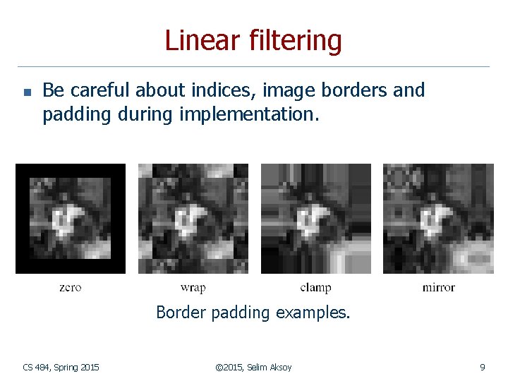
Linear filtering n Be careful about indices, image borders and padding during implementation. Border padding examples. CS 484, Spring 2015 © 2015, Selim Aksoy 9

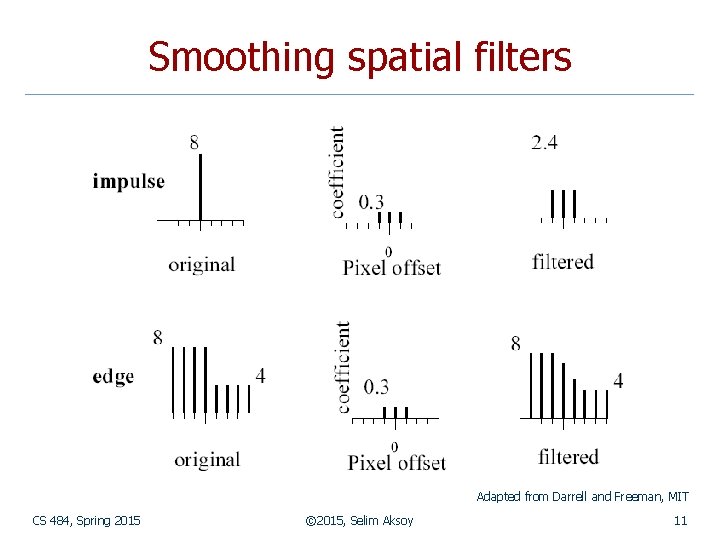
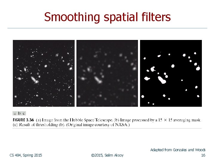
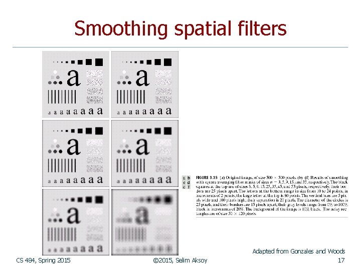
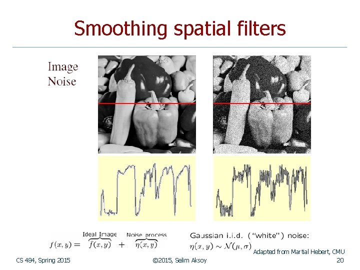
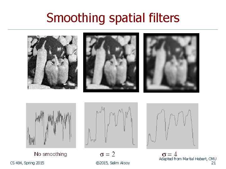
Smoothing spatial filters n Often, an image is composed of n n some underlying ideal structure, which we want to detect and describe, together with some random noise or artifact, which we would like to remove. Smoothing filters are used for blurring and for noise reduction. Linear smoothing filters are also called averaging filters. CS 484, Spring 2015 © 2015, Selim Aksoy 10

Smoothing spatial filters Adapted from Darrell and Freeman, MIT CS 484, Spring 2015 © 2015, Selim Aksoy 11

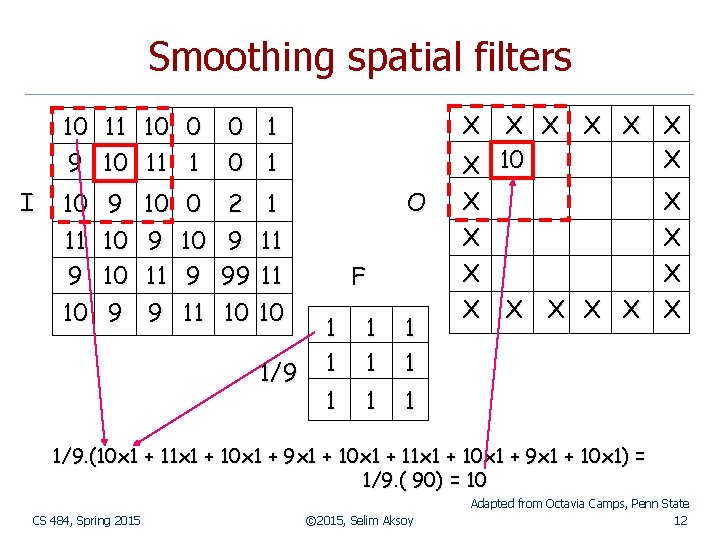
Smoothing spatial filters 10 9 I 11 10 10 11 0 1 10 9 10 0 X X X X 10 1 1 O 2 1 11 10 9 11 9 10 11 9 99 11 10 9 9 11 10 10 1/9 F 1 1 1 1 1 X X X 1/9. (10 x 1 + 11 x 1 + 10 x 1 + 9 x 1 + 10 x 1) = 1/9. ( 90) = 10 CS 484, Spring 2015 © 2015, Selim Aksoy Adapted from Octavia Camps, Penn State 12

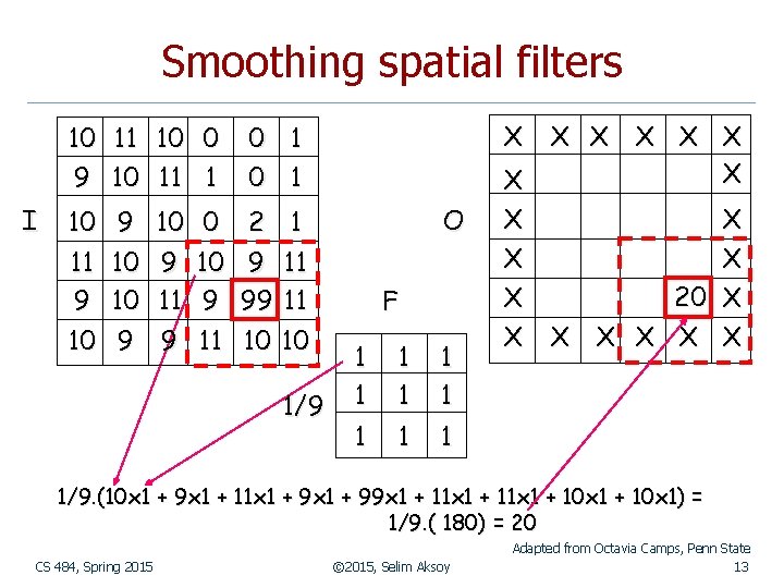
Smoothing spatial filters 10 9 I 11 10 10 11 0 1 10 9 10 0 X X X X 1 1 O 2 1 11 10 9 11 9 10 11 9 99 11 10 9 9 11 10 10 1/9 F 1 1 1 1 1 X X 20 X X X X 1/9. (10 x 1 + 9 x 1 + 11 x 1 + 99 x 1 + 11 x 1 + 10 x 1) = 1/9. ( 180) = 20 CS 484, Spring 2015 © 2015, Selim Aksoy Adapted from Octavia Camps, Penn State 13

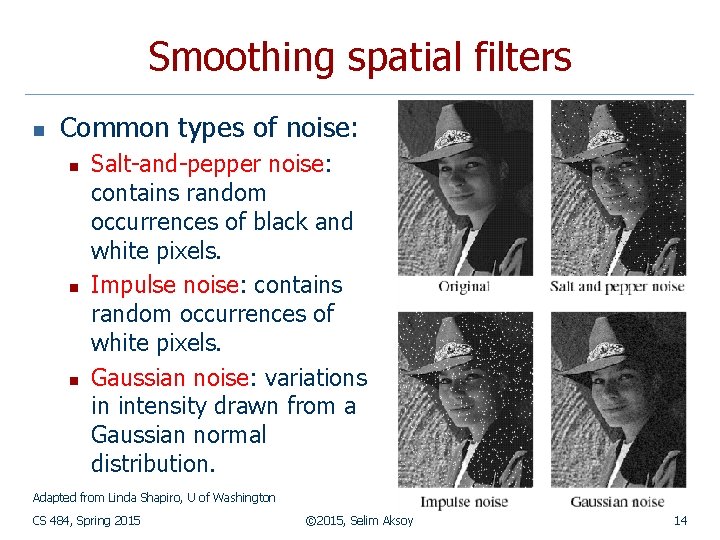
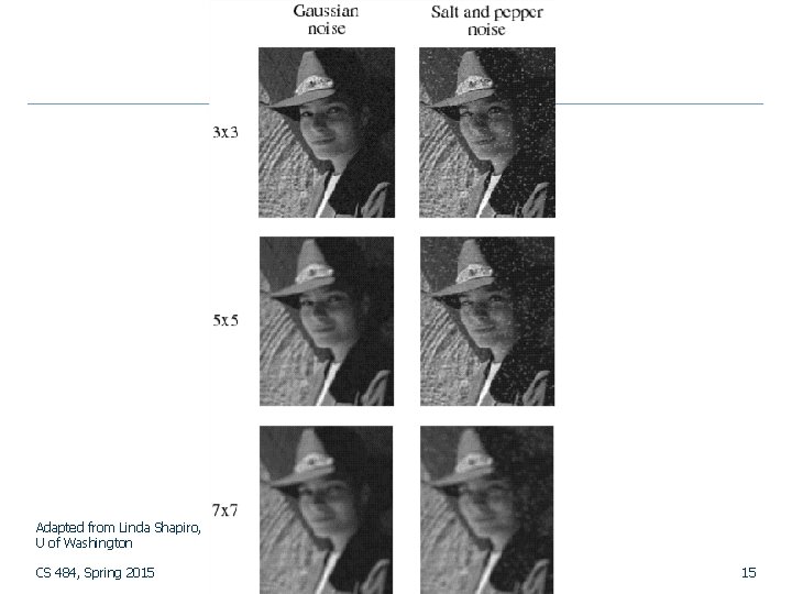
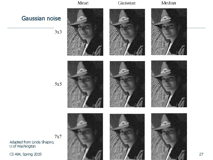
Smoothing spatial filters n Common types of noise: n n n Salt-and-pepper noise: contains random occurrences of black and white pixels. Impulse noise: contains random occurrences of white pixels. Gaussian noise: variations in intensity drawn from a Gaussian normal distribution. Adapted from Linda Shapiro, U of Washington CS 484, Spring 2015 © 2015, Selim Aksoy 14

Adapted from Linda Shapiro, U of Washington CS 484, Spring 2015 © 2015, Selim Aksoy 15

Smoothing spatial filters Adapted from Gonzales and Woods CS 484, Spring 2015 © 2015, Selim Aksoy 16

Smoothing spatial filters Adapted from Gonzales and Woods CS 484, Spring 2015 © 2015, Selim Aksoy 17

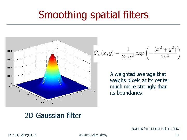
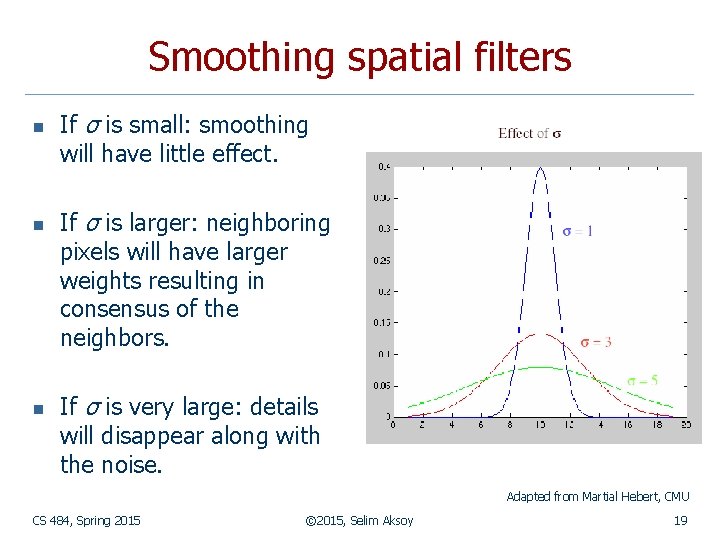
Smoothing spatial filters A weighted average that weighs pixels at its center much more strongly than its boundaries. 2 D Gaussian filter Adapted from Martial Hebert, CMU CS 484, Spring 2015 © 2015, Selim Aksoy 18

Smoothing spatial filters n n n If σ is small: smoothing will have little effect. If σ is larger: neighboring pixels will have larger weights resulting in consensus of the neighbors. If σ is very large: details will disappear along with the noise. Adapted from Martial Hebert, CMU CS 484, Spring 2015 © 2015, Selim Aksoy 19

Smoothing spatial filters CS 484, Spring 2015 © 2015, Selim Aksoy Adapted from Martial Hebert, CMU 20

Smoothing spatial filters CS 484, Spring 2015 © 2015, Selim Aksoy Adapted from Martial Hebert, CMU 21

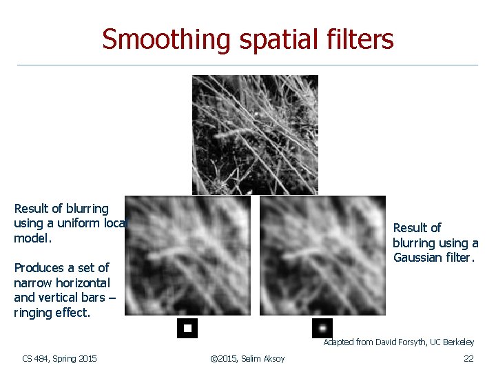
Smoothing spatial filters Result of blurring using a uniform local model. Result of blurring using a Gaussian filter. Produces a set of narrow horizontal and vertical bars – ringing effect. Adapted from David Forsyth, UC Berkeley CS 484, Spring 2015 © 2015, Selim Aksoy 22

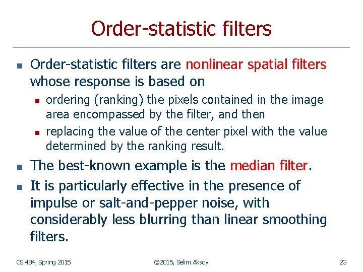
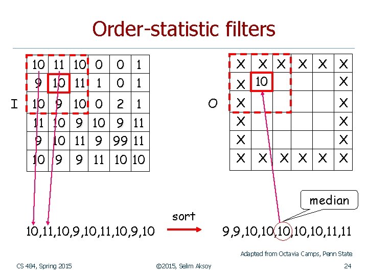
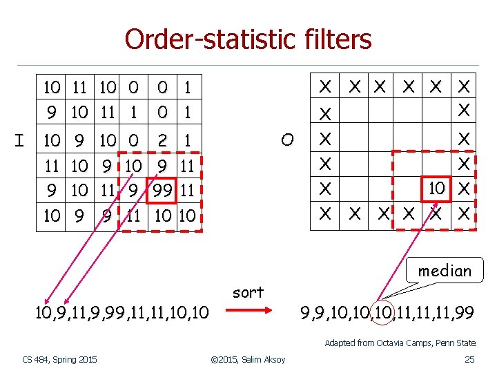
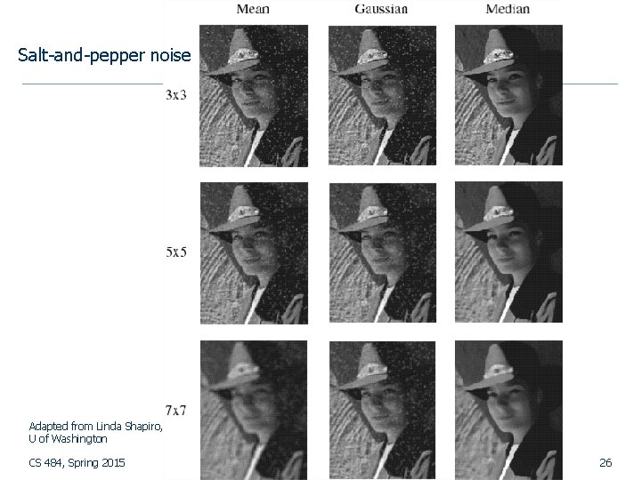
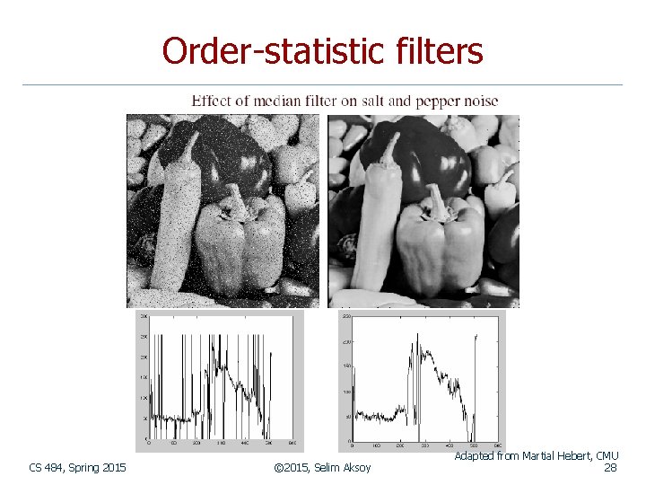
Order-statistic filters n Order-statistic filters are nonlinear spatial filters whose response is based on n n ordering (ranking) the pixels contained in the image area encompassed by the filter, and then replacing the value of the center pixel with the value determined by the ranking result. The best-known example is the median filter. It is particularly effective in the presence of impulse or salt-and-pepper noise, with considerably less blurring than linear smoothing filters. CS 484, Spring 2015 © 2015, Selim Aksoy 23

Order-statistic filters 10 9 I 11 10 10 11 0 1 10 9 10 0 X X X X 10 1 1 O 2 1 11 10 9 11 9 10 11 9 99 11 10 9 9 11 10 10 10, 11, 10, 9, 10 sort X X X median 9, 9, 10, 10, 10, 11 Adapted from Octavia Camps, Penn State CS 484, Spring 2015 © 2015, Selim Aksoy 24

Order-statistic filters 10 9 I 11 10 10 11 0 1 10 9 10 0 X X X X 1 1 O 2 1 11 10 9 11 9 10 11 9 99 11 10 9 9 11 10 10 10, 9, 11, 9, 99, 11, 10 sort X X 10 X X X X median 9, 9, 10, 10, 11, 11, 99 Adapted from Octavia Camps, Penn State CS 484, Spring 2015 © 2015, Selim Aksoy 25

Salt-and-pepper noise Adapted from Linda Shapiro, U of Washington CS 484, Spring 2015 © 2015, Selim Aksoy 26

Gaussian noise Adapted from Linda Shapiro, U of Washington CS 484, Spring 2015 © 2015, Selim Aksoy 27

Order-statistic filters CS 484, Spring 2015 © 2015, Selim Aksoy Adapted from Martial Hebert, CMU 28

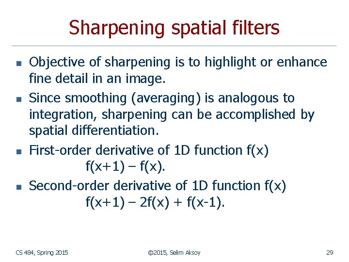
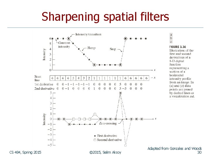
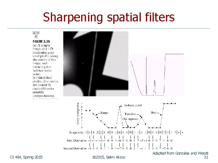
Sharpening spatial filters n n Objective of sharpening is to highlight or enhance fine detail in an image. Since smoothing (averaging) is analogous to integration, sharpening can be accomplished by spatial differentiation. First-order derivative of 1 D function f(x) f(x+1) – f(x). Second-order derivative of 1 D function f(x) f(x+1) – 2 f(x) + f(x-1). CS 484, Spring 2015 © 2015, Selim Aksoy 29

Sharpening spatial filters CS 484, Spring 2015 © 2015, Selim Aksoy Adapted from Gonzales and Woods 30

Sharpening spatial filters CS 484, Spring 2015 © 2015, Selim Aksoy Adapted from Gonzales and Woods 31

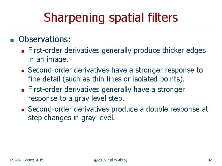
Sharpening spatial filters n Observations: n n First-order derivatives generally produce thicker edges in an image. Second-order derivatives have a stronger response to fine detail (such as thin lines or isolated points). First-order derivatives generally have a stronger response to a gray level step. Second-order derivatives produce a double response at step changes in gray level. CS 484, Spring 2015 © 2015, Selim Aksoy 32

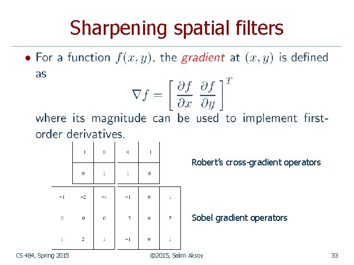
Sharpening spatial filters Robert’s cross-gradient operators Sobel gradient operators CS 484, Spring 2015 © 2015, Selim Aksoy 33

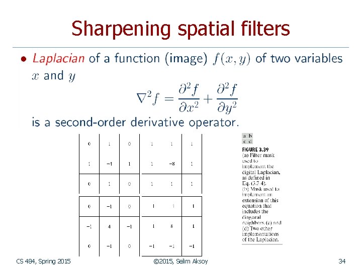
Sharpening spatial filters CS 484, Spring 2015 © 2015, Selim Aksoy 34

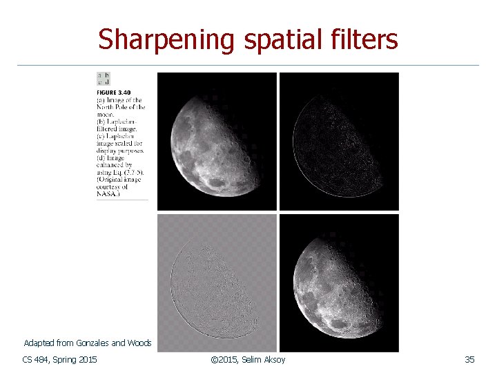
Sharpening spatial filters Adapted from Gonzales and Woods CS 484, Spring 2015 © 2015, Selim Aksoy 35

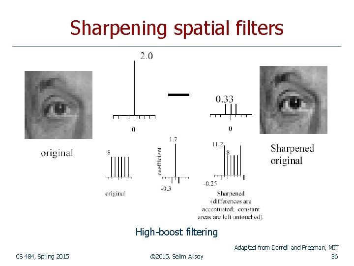
Sharpening spatial filters High-boost filtering Adapted from Darrell and Freeman, MIT CS 484, Spring 2015 © 2015, Selim Aksoy 36

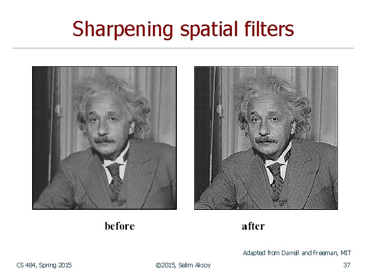
Sharpening spatial filters Adapted from Darrell and Freeman, MIT CS 484, Spring 2015 © 2015, Selim Aksoy 37

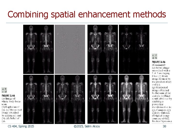
Combining spatial enhancement methods CS 484, Spring 2015 © 2015, Selim Aksoy 38