Texture Analysis Selim Aksoy Department of Computer Engineering

Texture Analysis Selim Aksoy Department of Computer Engineering Bilkent University saksoy@cs. bilkent. edu. tr

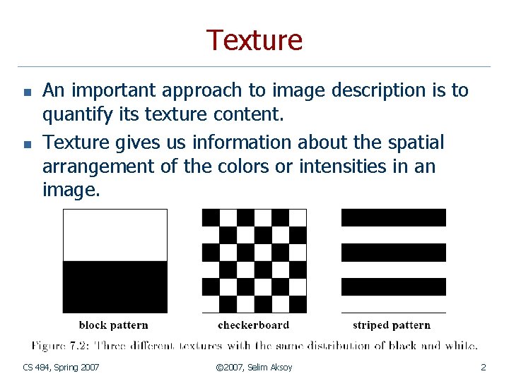
Texture n n An important approach to image description is to quantify its texture content. Texture gives us information about the spatial arrangement of the colors or intensities in an image. CS 484, Spring 2007 © 2007, Selim Aksoy 2

Texture n n Although no formal definition of texture exists, intuitively it can be defined as the uniformity, density, coarseness, roughness, regularity, intensity and directionality of discrete tonal features and their spatial relationships. Texture is commonly found in natural scenes, particularly in outdoor scenes containing both natural and man-made objects. CS 484, Spring 2007 © 2007, Selim Aksoy 3

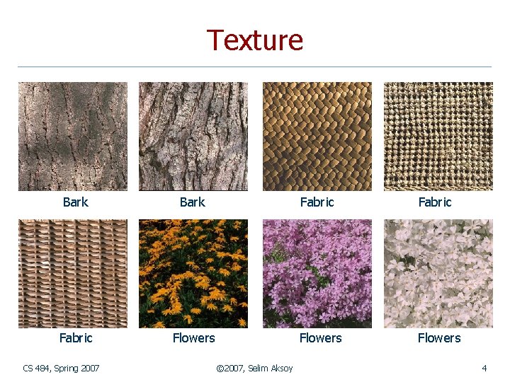
Texture Bark Fabric Flowers CS 484, Spring 2007 © 2007, Selim Aksoy 4

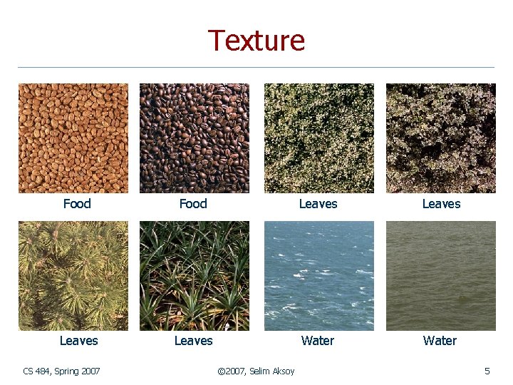
Texture Food Leaves Water CS 484, Spring 2007 © 2007, Selim Aksoy 5

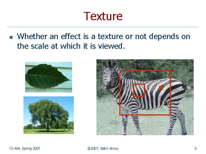
Texture n Whether an effect is a texture or not depends on the scale at which it is viewed. CS 484, Spring 2007 © 2007, Selim Aksoy 6

Texture n The approaches for characterizing and measuring texture can be grouped as: n n n structural approaches that use the idea that textures are made up of primitives appearing in a near-regular repetitive arrangement, statistical approaches that yield a quantitative measure of the arrangement of intensities. While the first approach is appealing and can work well for man-made, regular patterns, the second approach is more general and easier to compute and is used more often in practice. CS 484, Spring 2007 © 2007, Selim Aksoy 7

Structural approaches n n n Structural approaches model texture as a set of primitive texels (texture elements) in a particular spatial relationship. A structural description of a texture includes a description of the texels and a specification of the spatial relationship. Of course, the texels must be identifiable and the relationship must be efficiently computable. CS 484, Spring 2007 © 2007, Selim Aksoy 8

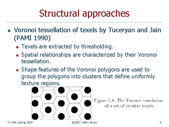
Structural approaches n Voronoi tessellation of texels by Tuceryan and Jain (PAMI 1990) n n n Texels are extracted by thresholding. Spatial relationships are characterized by their Voronoi tessellation. Shape features of the Voronoi polygons are used to group the polygons into clusters that define uniformly texture regions. CS 484, Spring 2007 © 2007, Selim Aksoy 9

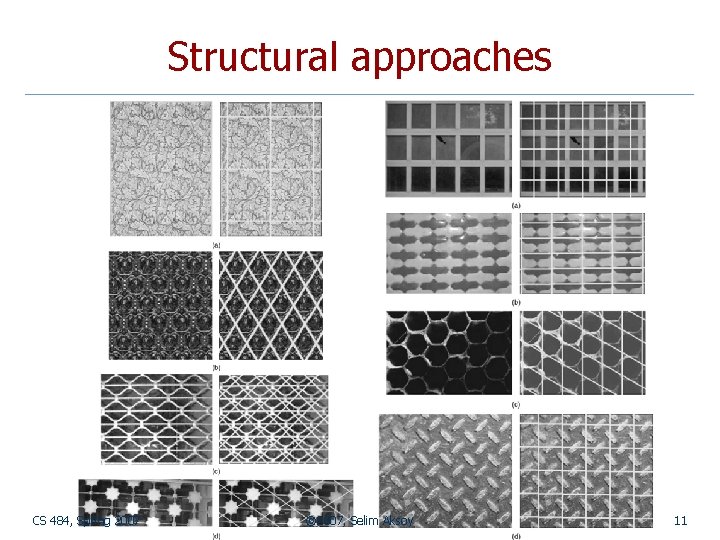
Structural approaches n Computational model for periodic pattern perception based on frieze and wallpaper groups by Liu, Collins and Tsin (PAMI 2004) n n A frieze pattern is a 2 D strip in the plane that is periodic along one dimension. A periodic pattern extended in two linearly independent directions to cover the 2 D plane is known as a wallpaper pattern. CS 484, Spring 2007 © 2007, Selim Aksoy 10

Structural approaches CS 484, Spring 2007 © 2007, Selim Aksoy 11

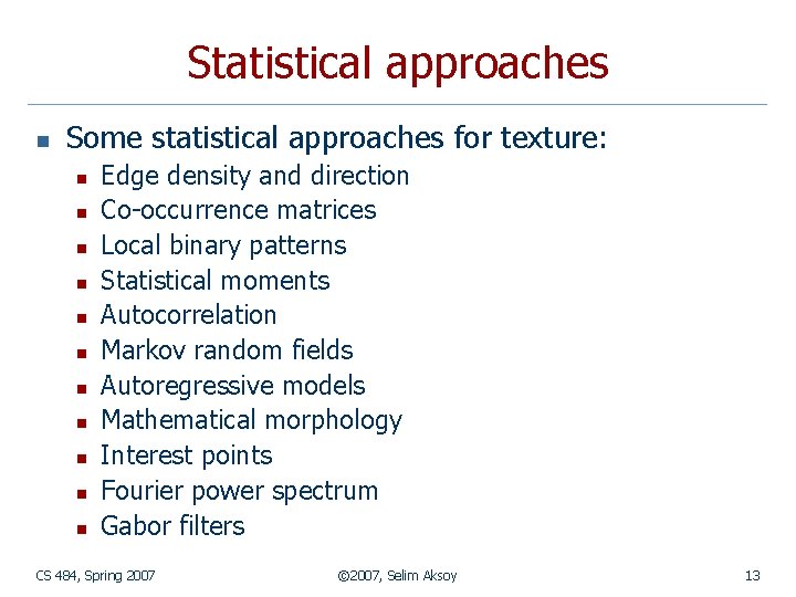
Statistical approaches n n n Usually, segmenting out the texels is difficult or impossible in real images. Instead, numeric quantities or statistics that describe a texture can be computed from the gray tones or colors themselves. This approach is less intuitive, but is computationally efficient and often works well. CS 484, Spring 2007 © 2007, Selim Aksoy 12

Statistical approaches n Some statistical approaches for texture: n n n Edge density and direction Co-occurrence matrices Local binary patterns Statistical moments Autocorrelation Markov random fields Autoregressive models Mathematical morphology Interest points Fourier power spectrum Gabor filters CS 484, Spring 2007 © 2007, Selim Aksoy 13

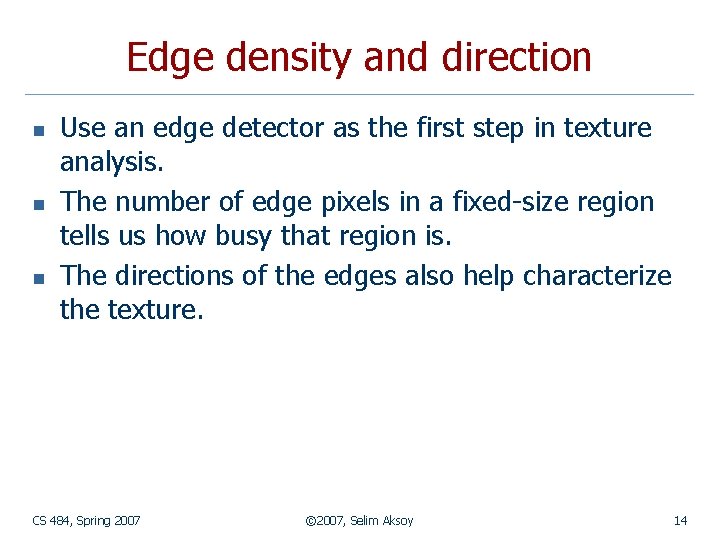
Edge density and direction n Use an edge detector as the first step in texture analysis. The number of edge pixels in a fixed-size region tells us how busy that region is. The directions of the edges also help characterize the texture. CS 484, Spring 2007 © 2007, Selim Aksoy 14

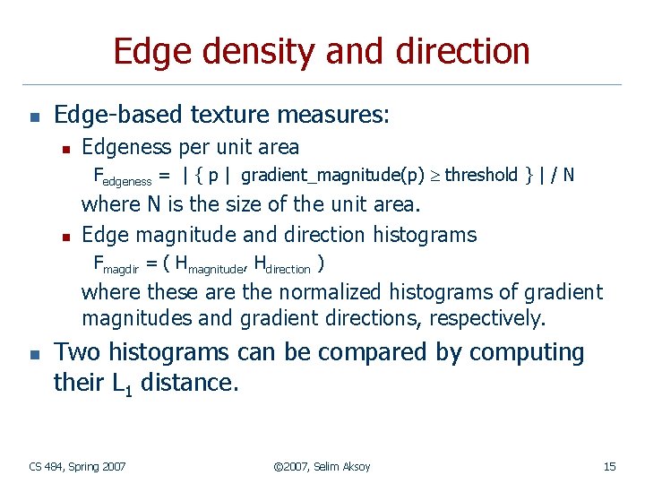
Edge density and direction n Edge-based texture measures: n Edgeness per unit area Fedgeness = | { p | gradient_magnitude(p) threshold } | / N n where N is the size of the unit area. Edge magnitude and direction histograms Fmagdir = ( Hmagnitude, Hdirection ) where these are the normalized histograms of gradient magnitudes and gradient directions, respectively. n Two histograms can be compared by computing their L 1 distance. CS 484, Spring 2007 © 2007, Selim Aksoy 15

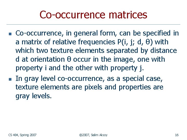
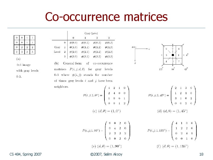
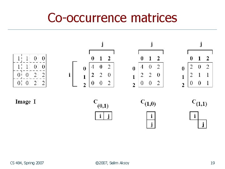
Co-occurrence matrices n n Co-occurrence, in general form, can be specified in a matrix of relative frequencies P(i, j; d, θ) with which two texture elements separated by distance d at orientation θ occur in the image, one with property i and the other with property j. In gray level co-occurrence, as a special case, texture elements are pixels and properties are gray levels. CS 484, Spring 2007 © 2007, Selim Aksoy 16

Co-occurrence matrices n n The spatial relationship can also be specified as a displacement vector (dr, dc) where dr is a displacement in rows and dc is a displacement in columns. For a particular displacement, the resulting square matrix can be normalized by dividing each entry by the number of elements used to compute that matrix. CS 484, Spring 2007 © 2007, Selim Aksoy 17

Co-occurrence matrices CS 484, Spring 2007 © 2007, Selim Aksoy 18

Co-occurrence matrices CS 484, Spring 2007 © 2007, Selim Aksoy 19

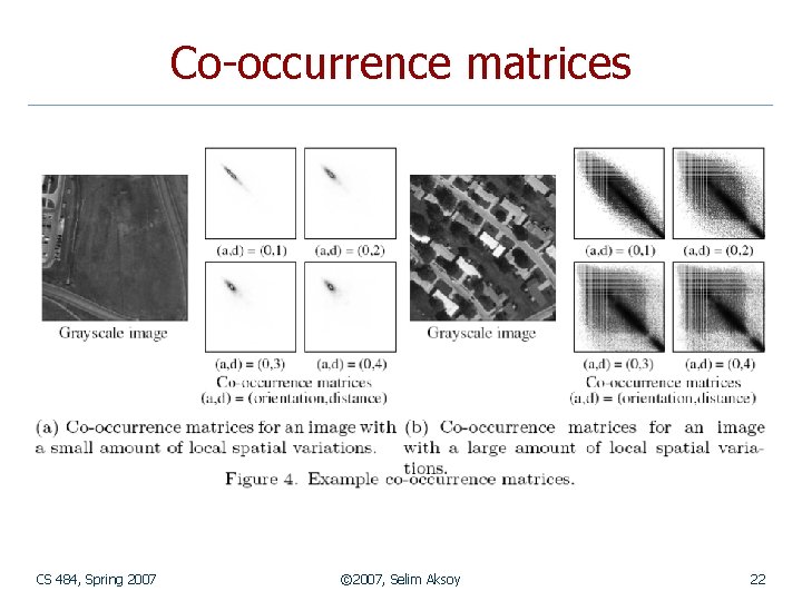
Co-occurrence matrices n n n If a texture is coarse and the distance d used to compute the co-occurrence matrix is small compared to the sizes of the texture elements, pairs of pixels at separation d should usually have similar gray levels. This means that high values in the matrix P(i, j; d, θ) should be concentrated on or near its main diagonal. Conversely, for a fine texture, if d is comparable to the texture element size, then the gray levels of points separated by d should often be quite different, so that values in P(i, j; d, θ) should be spread out relatively uniformly. CS 484, Spring 2007 © 2007, Selim Aksoy 20

Co-occurrence matrices n n Similarly, if a texture is directional, i. e. , coarser in one direction than another, the degree of spread of the values about the main diagonal in P(i, j; d, θ) should vary with the orientation θ. Thus texture directionality can be analyzed by comparing spread measures of P(i, j; d, θ) for various orientations. CS 484, Spring 2007 © 2007, Selim Aksoy 21

Co-occurrence matrices CS 484, Spring 2007 © 2007, Selim Aksoy 22

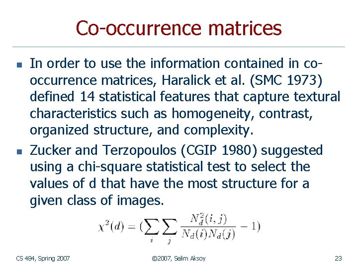
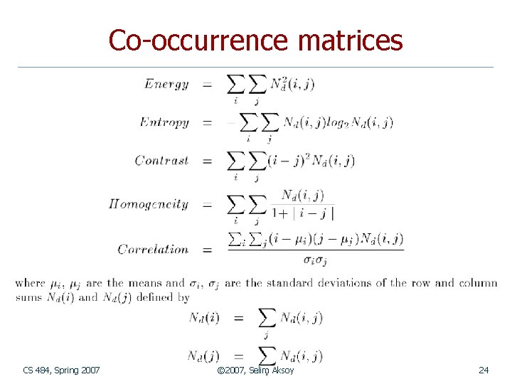
Co-occurrence matrices n n In order to use the information contained in cooccurrence matrices, Haralick et al. (SMC 1973) defined 14 statistical features that capture textural characteristics such as homogeneity, contrast, organized structure, and complexity. Zucker and Terzopoulos (CGIP 1980) suggested using a chi-square statistical test to select the values of d that have the most structure for a given class of images. CS 484, Spring 2007 © 2007, Selim Aksoy 23

Co-occurrence matrices CS 484, Spring 2007 © 2007, Selim Aksoy 24

Co-occurrence matrices Example building groups (first column), the contrast features for 0 and 67. 5 degree orientations (second and third columns), and the chi-square features for 0 and 67. 5 degree orientations (fourth and fifth columns). X-axes represent inter-pixel distances of 1 to 60. The features at a particular orientation exhibit a periodic structure as a function of distance if the neighborhood contains a regular arrangement of buildings along that direction. On the other hand, features are very similar for different orientations if there is no particular arrangement in the neighborhood. CS 484, Spring 2007 © 2007, Selim Aksoy 25

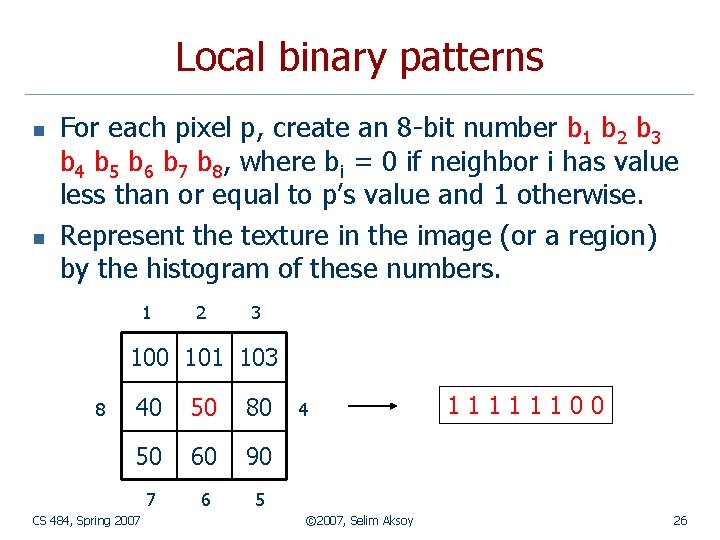
Local binary patterns n n For each pixel p, create an 8 -bit number b 1 b 2 b 3 b 4 b 5 b 6 b 7 b 8, where bi = 0 if neighbor i has value less than or equal to p’s value and 1 otherwise. Represent the texture in the image (or a region) by the histogram of these numbers. 1 2 3 100 101 103 8 40 50 80 50 60 90 7 6 5 CS 484, Spring 2007 4 © 2007, Selim Aksoy 11111100 26

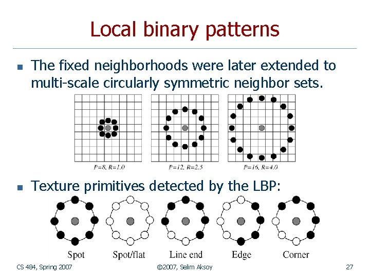
Local binary patterns n n The fixed neighborhoods were later extended to multi-scale circularly symmetric neighbor sets. Texture primitives detected by the LBP: CS 484, Spring 2007 © 2007, Selim Aksoy 27

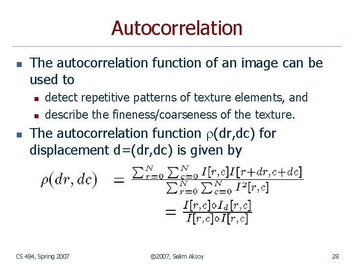
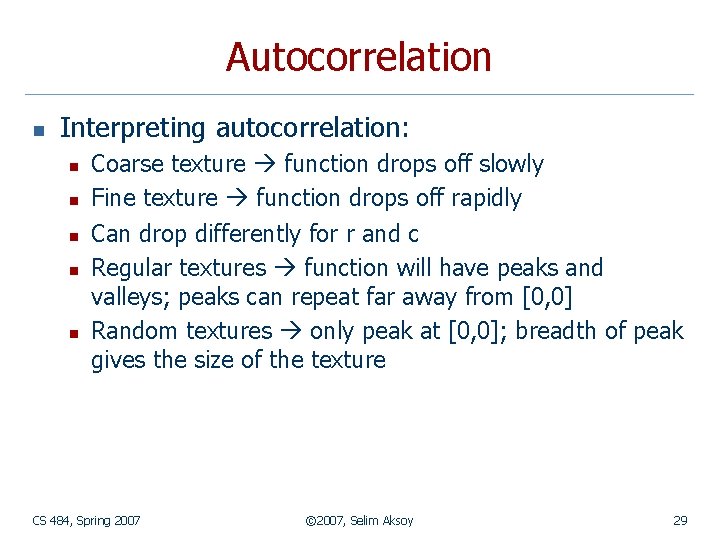
Autocorrelation n The autocorrelation function of an image can be used to n n n detect repetitive patterns of texture elements, and describe the fineness/coarseness of the texture. The autocorrelation function (dr, dc) for displacement d=(dr, dc) is given by CS 484, Spring 2007 © 2007, Selim Aksoy 28

Autocorrelation n Interpreting autocorrelation: n n n Coarse texture function drops off slowly Fine texture function drops off rapidly Can drop differently for r and c Regular textures function will have peaks and valleys; peaks can repeat far away from [0, 0] Random textures only peak at [0, 0]; breadth of peak gives the size of the texture CS 484, Spring 2007 © 2007, Selim Aksoy 29

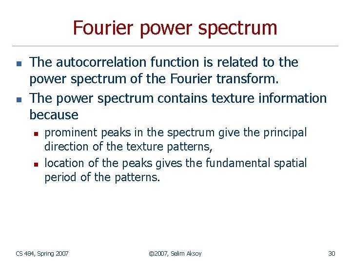
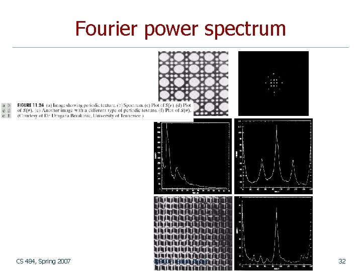
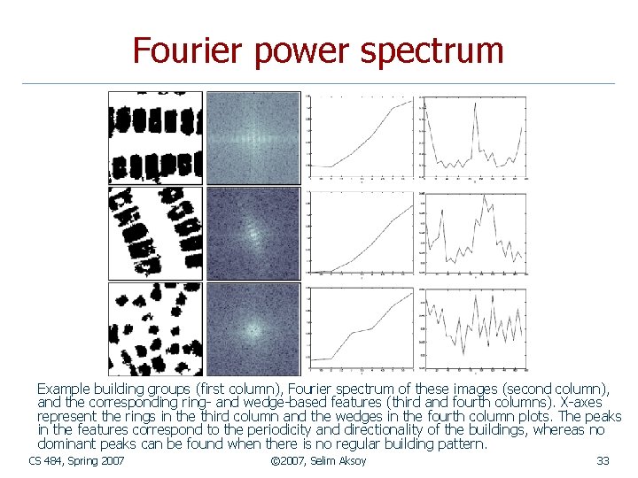
Fourier power spectrum n n The autocorrelation function is related to the power spectrum of the Fourier transform. The power spectrum contains texture information because n n prominent peaks in the spectrum give the principal direction of the texture patterns, location of the peaks gives the fundamental spatial period of the patterns. CS 484, Spring 2007 © 2007, Selim Aksoy 30

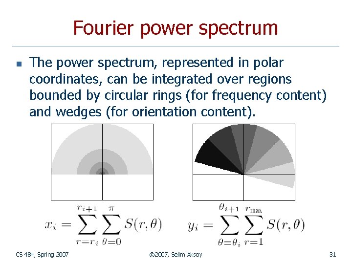
Fourier power spectrum n The power spectrum, represented in polar coordinates, can be integrated over regions bounded by circular rings (for frequency content) and wedges (for orientation content). CS 484, Spring 2007 © 2007, Selim Aksoy 31

Fourier power spectrum CS 484, Spring 2007 © 2007, Selim Aksoy 32

Fourier power spectrum Example building groups (first column), Fourier spectrum of these images (second column), and the corresponding ring- and wedge-based features (third and fourth columns). X-axes represent the rings in the third column and the wedges in the fourth column plots. The peaks in the features correspond to the periodicity and directionality of the buildings, whereas no dominant peaks can be found when there is no regular building pattern. CS 484, Spring 2007 © 2007, Selim Aksoy 33

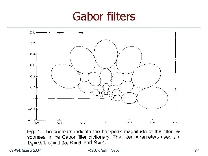
Gabor filters n n n The Gabor representation has been shown to be optimal in the sense of minimizing the joint twodimensional uncertainty in space and frequency. These filters can be considered as orientation and scale tunable edge and line detectors. Fourier transform achieves localization in either spatial or frequency domain but the Gabor transform achieves simultaneous localization in both spatial and frequency domains. CS 484, Spring 2007 © 2007, Selim Aksoy 34

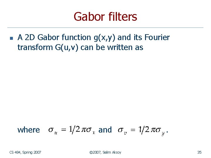
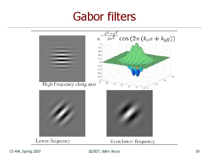
Gabor filters n A 2 D Gabor function g(x, y) and its Fourier transform G(u, v) can be written as where CS 484, Spring 2007 and © 2007, Selim Aksoy . 35

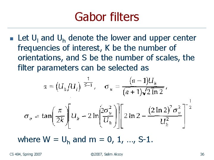
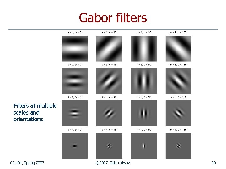
Gabor filters n Let Ul and Uh denote the lower and upper center frequencies of interest, K be the number of orientations, and S be the number of scales, the filter parameters can be selected as where W = Uh and m = 0, 1, …, S-1. CS 484, Spring 2007 © 2007, Selim Aksoy 36

Gabor filters CS 484, Spring 2007 © 2007, Selim Aksoy 37

Gabor filters Filters at multiple scales and orientations. CS 484, Spring 2007 © 2007, Selim Aksoy 38

Gabor filters CS 484, Spring 2007 © 2007, Selim Aksoy 39

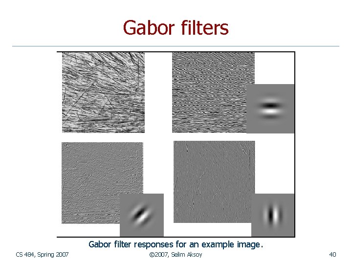
Gabor filters Gabor filter responses for an example image. CS 484, Spring 2007 © 2007, Selim Aksoy 40

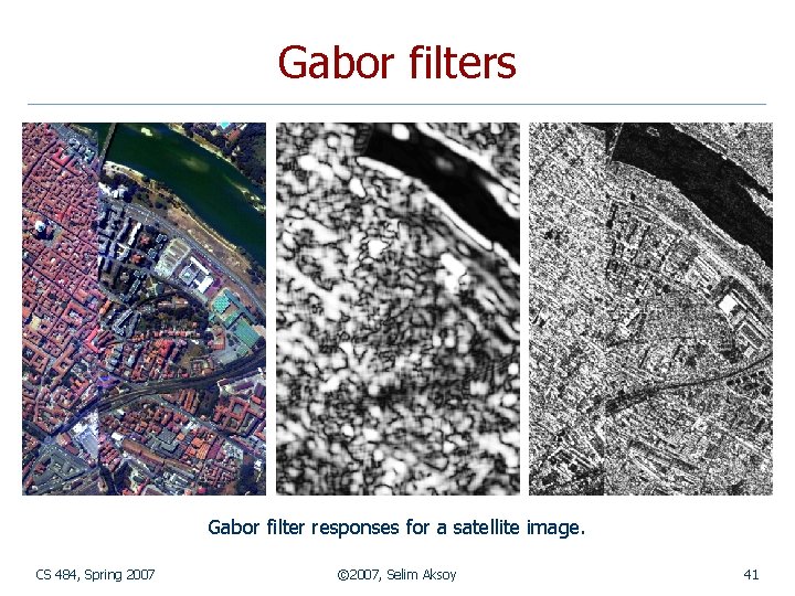
Gabor filters Gabor filter responses for a satellite image. CS 484, Spring 2007 © 2007, Selim Aksoy 41

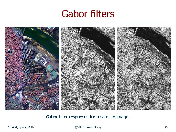
Gabor filters Gabor filter responses for a satellite image. CS 484, Spring 2007 © 2007, Selim Aksoy 42

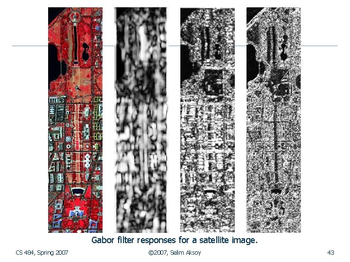
Gabor filter responses for a satellite image. CS 484, Spring 2007 © 2007, Selim Aksoy 43

CS 484, Spring 2007 © 2007, Selim Aksoy 44

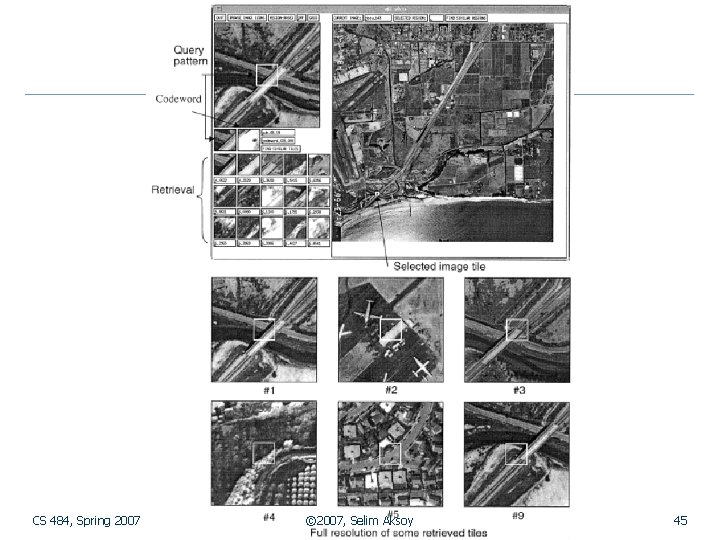
CS 484, Spring 2007 © 2007, Selim Aksoy 45

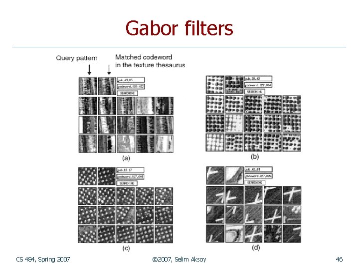
Gabor filters CS 484, Spring 2007 © 2007, Selim Aksoy 46

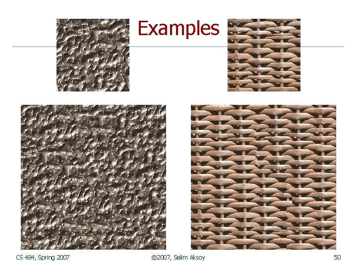
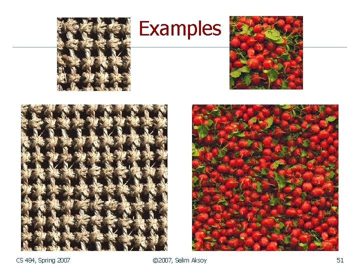
Texture synthesis n n Goal of texture analysis: compare textures and decide if they are similar. Goal of texture synthesis: construct large regions of texture from small example images. It is an important problem for rendering in computer graphics. Strategy: to think of a texture as a sample from some probability distribution and then to try and obtain other samples from that same distribution. CS 484, Spring 2007 © 2007, Selim Aksoy 47

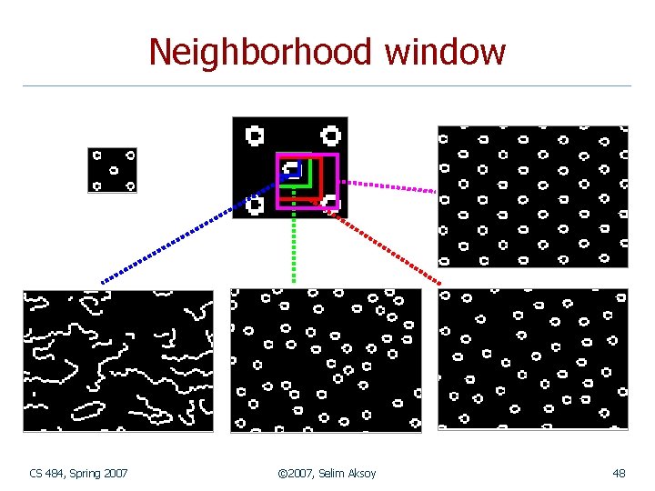
Neighborhood window CS 484, Spring 2007 © 2007, Selim Aksoy 48

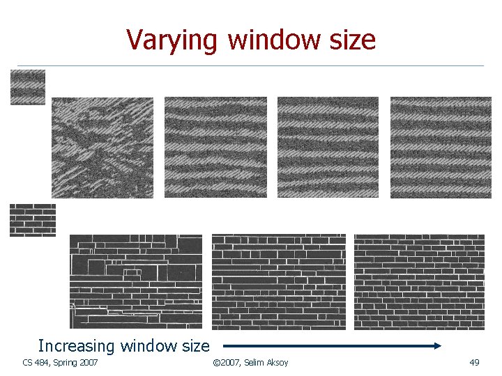
Varying window size Increasing window size CS 484, Spring 2007 © 2007, Selim Aksoy 49

Examples CS 484, Spring 2007 © 2007, Selim Aksoy 50

Examples CS 484, Spring 2007 © 2007, Selim Aksoy 51

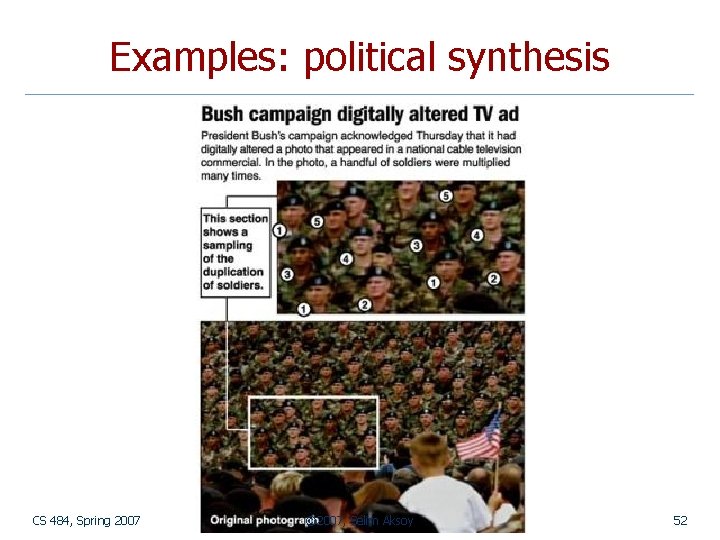
Examples: political synthesis CS 484, Spring 2007 © 2007, Selim Aksoy 52

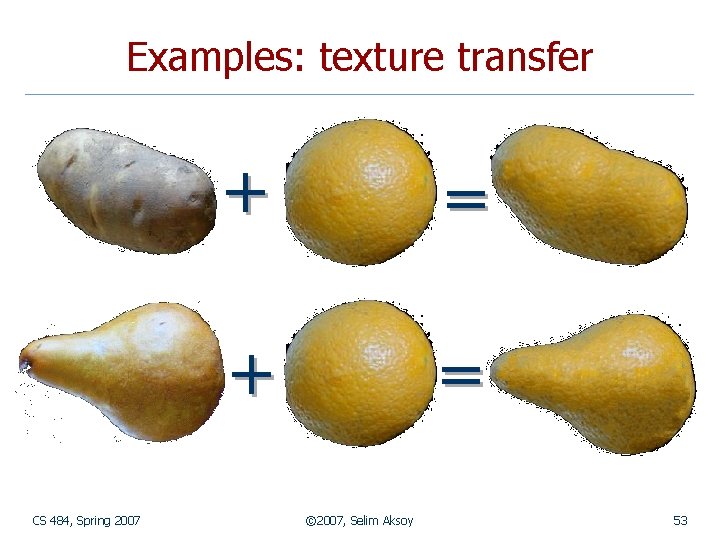
Examples: texture transfer CS 484, Spring 2007 + = © 2007, Selim Aksoy 53

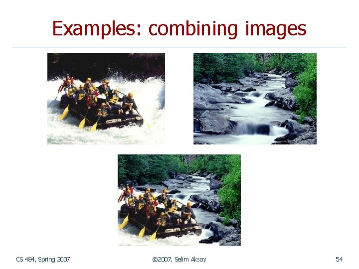
Examples: combining images CS 484, Spring 2007 © 2007, Selim Aksoy 54

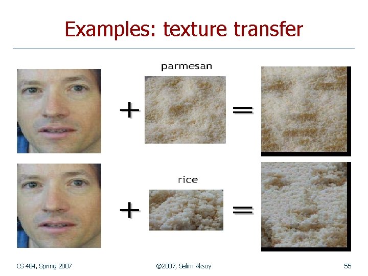
Examples: texture transfer CS 484, Spring 2007 © 2007, Selim Aksoy 55

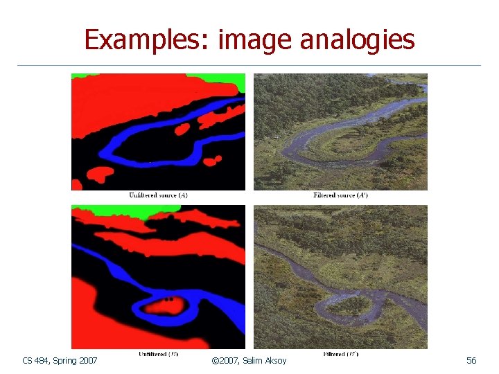
Examples: image analogies CS 484, Spring 2007 © 2007, Selim Aksoy 56

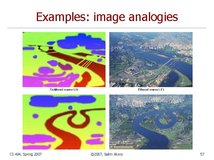
Examples: image analogies CS 484, Spring 2007 © 2007, Selim Aksoy 57