Lecture Slides for INTRODUCTION TO Machine Learning 2

Lecture Slides for INTRODUCTION TO Machine Learning 2 nd Edition ETHEM ALPAYDIN © The MIT Press, 2010 alpaydin@boun. edu. tr http: //www. cmpe. boun. edu. tr/~ethem/i 2 ml 2 e

CHAPTER 7: Clustering

Semiparametric Density Estimation �Parametric: Assume a single model for p(x|Ci) (Chapter 4 and 5) �Semiparametric: p(x|Ci) is a mixture of densities Multiple possible explanations/prototypes: Different handwriting styles, accents in speech �Nonparametric: No model; data speaks for itself (Chapter 8) Lecture Notes for E Alpaydın 2010 Introduction to Machine Learning 2 e © The MIT Press (V 1. 0) 3

Mixture Densities where Gi : the mixture components/groups/clusters P(Gi) : mixture proportions (priors) p(x|Gi) : component densities Gaussian mixture where p(x|Gi) ~ N ( μi , ∑i ) parameters Φ = {P(Gi ), μi , ∑i }ki=1 unlabeled sample X={xt}Nt=1 (unsupervised learning) Lecture Notes for E Alpaydın 2010 Introduction to Machine Learning 2 e © The MIT Press (V 1. 0) 4

Classes vs. Clusters Supervised: X = { xt , rt }t Classes Ci , i =1, . . . , K Unsupervised : X = { xt }t Clusters Gi , i =1, . . . , k where p(x|Ci)~N (μi, ∑i ) where p(x|Gi)~N (μi, ∑i) Φ = {P(Ci ), μi , ∑i }Ki=1 Φ = {P(Gi ), μi , ∑i }ki=1 Labels, r ti ? Lecture Notes for E Alpaydın 2010 Introduction to Machine Learning 2 e © The MIT Press (V 1. 0) 5

k-Means Clustering �Find k reference vectors (prototypes/codebook vectors/ codewords) which best represent data �Reference vectors, mj, j =1, . . . , k �Use nearest (most similar) reference: �Reconstruction error Lecture Notes for E Alpaydın 2010 Introduction to Machine Learning 2 e © The MIT Press (V 1. 0) 6

Lecture Notes for E Alpaydın 2010 Introduction to Machine Learning 2 e © The MIT Press (V 1. 0) 7

k-means Clustering Lecture Notes for E Alpaydın 2010 Introduction to Machine Learning 2 e © The MIT Press (V 1. 0) 8

k-means Clustering � One disadvantage: � A local search procedure � The final mi highly depend on the initial mi � The methods to initial mi � Randomly select k instances � Calculate the mean of all data and add small random vectors � Calculate the principal component partitioning the data into k groups, and then take the means of these groups Lecture Notes for E Alpaydın 2010 Introduction to Machine Learning 2 e © The MIT Press (V 1. 0) 9

Encoding/Decoding Lecture Notes for E Alpaydın 2010 Introduction to Machine Learning 2 e © The MIT Press (V 1. 0) 10

11 Expectation-Maximization Algorithm • An expectation-maximization (EM) algorithm is used in statistics for finding maximum likelihood estimates of parameters in probabilistic models, where the model depends on unobserved latent variables. • EM is an iterative method which alternates between performing an expectation (E) step, ▫ which computes an expectation of the log likelihood with respect to the current estimate of the distribution for the latent variables, and a maximization (M) step, ▫ which computes the parameters which maximize the expected log likelihood found on the E step. (http: //en. wikipedia. org/wiki/Expectation-maximization_algorithm)

Expectation-Maximization (EM) � Log likelihood with a mixture model � Assume hidden variables z, which when known, make optimization much simpler � Complete likelihood, Lc(Φ |X, Z), in terms of x and z � Incomplete likelihood, L(Φ |X), in terms of x Lecture Notes for E Alpaydın 2010 Introduction to Machine Learning 2 e © The MIT Press (V 1. 0) 12

E- and M-steps � Iterate the two steps 1. E-step: Estimate the expectation of the log likelihood given X and current Φ 2. M-step: Find new Φ’ given z, X, and old Φ. An increase in Q increases incomplete likelihood (proven by Laird and Rubin (1977)) Lecture Notes for E Alpaydın 2010 Introduction to Machine Learning 2 e © The MIT Press (V 1. 0) 13

EM in Gaussian Mixtures �Define indicator variables zt ={zt 1 , zt 2 , …, ztk } zti = 1 if xt belongs to Gi, 0 otherwise; assume p(x|Gi)~N(μi, ∑i) �z is the multinomial distribution from k categories with prior probabilities πi. �E-step: (See p. 169 - p. 170) where Lecture Notes for E Alpaydın 2010 Introduction to Machine Learning 2 e © The MIT Press (V 1. 0) 14

EM in Gaussian Mixtures �M-step: assume p(x|Gi)~N(mi, Si), the M-step is (see p. 170) Use estimated labels in place of unknown labels Lecture Notes for E Alpaydın 2010 Introduction to Machine Learning 2 e © The MIT Press (V 1. 0) 15

EM in Gaussian Mixtures �E-step: Lecture Notes for E Alpaydın 2010 Introduction to Machine Learning 2 e © The MIT Press (V 1. 0) 16

P(Gi|x)=hi=0. 5 Data points and the fitted Gaussians by EM, initialized by one k-means iteration of Figure 7. 2. Unlike in k-means, EM allows estimating the covariance matrices. hi indicates the contours of the estimated Gaussian densities. Lecture Notes for E Alpaydın 2010 Introduction to Machine Learning 2 e © The MIT Press (V 1. 0) 17

Discussion � If the input dimensionality is high and the sample is small, to decrease the number of parameters: � Assuming a common covariance matrix may not be right since clusters may really have different shapes. � Assuming diagonal matrices is even more risky because it removes all correlations. � The alternative is to do dimensionality reduction in the clusters. � Use PCA/FA to decrease dimensionality. (Ghahramani and Hinton, 1997; Tipping and Bishop, 1999) � For example, in mixtures of FA use EM to learn Vi. Vi and specific variances of cluster are the factor loadings and. Lecture Notes for E Alpaydın 2010 Introduction to Machine Learning 2 e © The MIT Press (V 1. 0) 18

Supervised Learning after Clustering �Dimensionality reduction methods find correlations between variables and thus group variables. �Clustering methods find similarities between instances and thus group instances. �Allows knowledge extraction through number of clusters, prior probabilities, cluster parameters, i. e. , center, range of features. Example: customer segmentation Lecture Notes for E Alpaydın 2010 Introduction to Machine Learning 2 e © The MIT Press (V 1. 0) 19

Mixture of Mixtures �In classification, the input comes from a mixture of classes (supervised). �If each class is also a mixture, e. g. , of Gaussians, (unsupervised), we have a mixture of mixtures: Lecture Notes for E Alpaydın 2010 Introduction to Machine Learning 2 e © The MIT Press (V 1. 0) 20

Hierarchical Clustering �Cluster based on similarities/distances �Distance measure between instances xr and xs Minkowski distance (Lp) (Euclidean for p = 2) City-block distance Lecture Notes for E Alpaydın 2010 Introduction to Machine Learning 2 e © The MIT Press (V 1. 0) 21

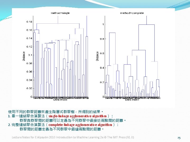
Agglomerative(會凝聚的) Clustering �Start with N groups each with one instance and merge two closest groups at each iteration �Distance between two groups Gi and Gj: �Single-link clustering: �Complete-link clustering: �Average-link clustering, centroid Lecture Notes for E Alpaydın 2010 Introduction to Machine Learning 2 e © The MIT Press (V 1. 0) 22

Example: Single-Link Clustering Dendrogram(樹狀圖) Lecture Notes for E Alpaydın 2010 Introduction to Machine Learning 2 e © The MIT Press (V 1. 0) 23

http: //mirlab. org/jang/books/dcpr/dc. Hier. Clustering. asp? title=32%20 Hierarchical%20 Clustering%20(%B 6%A 5%BCh%A 6%A 1%A 4%C 0%B 8 s%AAk)&language=chinese Lecture Notes for E Alpaydın 2010 Introduction to Machine Learning 2 e © The MIT Press (V 1. 0) 24

Choosing k (the number of clusters) �Defined by the application �e. g. , image quantization �Plot data (after PCA) and check for clusters �Incremental (leader-cluster) algorithm �Add one at a time until “elbow” (reconstruction error/log likelihood/intergroup distances) �Manual check for meaning Lecture Notes for E Alpaydın 2010 Introduction to Machine Learning 2 e © The MIT Press (V 1. 0) 26

Exercises �What are the similarities and difference between average-link clustering and k-means? �How can we make k-means robust to outliers? Lecture Notes for E Alpaydın 2010 Introduction to Machine Learning 2 e © The MIT Press (V 1. 0) 27