Lecture 6 Linear Programming Sensitivity Analysis OSCM 230

Lecture 6 Linear Programming: Sensitivity Analysis OSCM 230 Fall 2013 Management Science Lecture 6 Linear Programming Sensitivity Analysis 9/23/2013, 9/25/2013 Professor Dong Washington University in St. Louis, MO 1

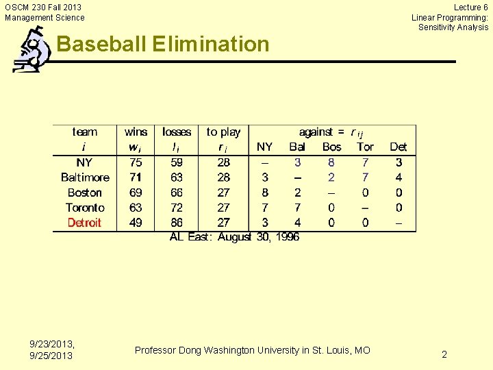
OSCM 230 Fall 2013 Management Science Baseball Elimination 9/23/2013, 9/25/2013 Professor Dong Washington University in St. Louis, MO Lecture 6 Linear Programming: Sensitivity Analysis 2

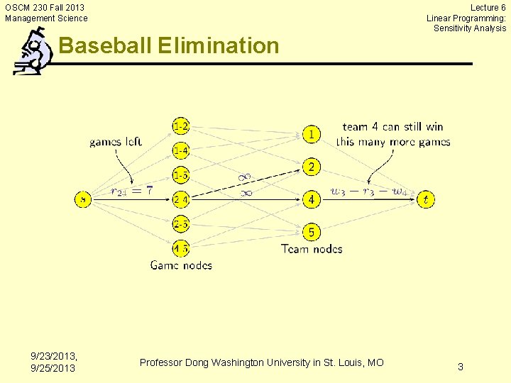
OSCM 230 Fall 2013 Management Science Baseball Elimination 9/23/2013, 9/25/2013 Professor Dong Washington University in St. Louis, MO Lecture 6 Linear Programming: Sensitivity Analysis 3

OSCM 230 Fall 2013 Management Science Introduction Lecture 6 Linear Programming: Sensitivity Analysis • In general, we are never content with only the optimal solution to a linear program and want to acquire insight into the economics of the situation we are modeling • For example, we may want to know how sensitive our solution is to changes in the objective function or changes in some of the constraints. (Why? ) • Frequently, firms may want to invest in order to alleviate constraints: how exactly should a potential investment be allocated • Sensitivity analysis is vital to the intelligent use of any optimal LP solution 9/23/2013, 9/25/2013 Professor Dong Washington University in St. Louis, MO 4

OSCM 230 Fall 2013 Management Science Introduction Lecture 6 Linear Programming: Sensitivity Analysis • The first part of the lecture gives an “operational overview” of the most important concepts in sensitivity analysis. • In the first part, we’ll learn “how to” using Excel output • Then we’ll try to dig deeper and explore some of the “why” questions • For example, we’ll learn that sensitivity analysis offers a unique insight into the properties of the optimal solution of any linear program 9/23/2013, 9/25/2013 Professor Dong Washington University in St. Louis, MO 5

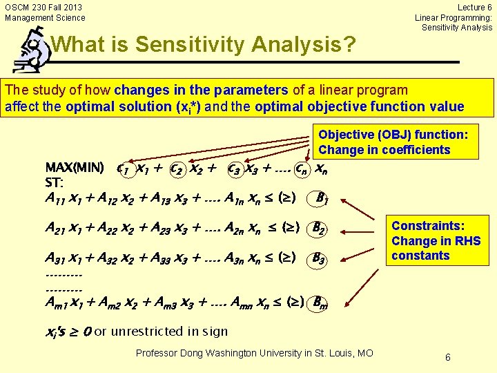
OSCM 230 Fall 2013 Management Science What is Sensitivity Analysis? Lecture 6 Linear Programming: Sensitivity Analysis The study of how changes in the parameters of a linear program affect the optimal solution (xi*) and the optimal objective function value Objective (OBJ) function: Change in coefficients MAX(MIN) c 1 x 1 + c 2 x 2 + c 3 x 3 + …. cn xn ST: A 11 x 1 + A 12 x 2 + A 13 x 3 + …. A 1 n xn ≤ (≥) B 1 A 21 x 1 + A 22 x 2 + A 23 x 3 + …. A 2 n xn ≤ (≥) B 2 A 31 x 1 + A 32 x 2 + A 33 x 3 + …. A 3 n xn ≤ (≥) B 3 ……… Am 1 x 1 + Am 2 x 2 + Am 3 x 3 + …. Amn xn ≤ (≥) Bm Constraints: Change in RHS constants xi's ≥ 0 or unrestricted in sign Professor Dong Washington University in St. Louis, MO 6

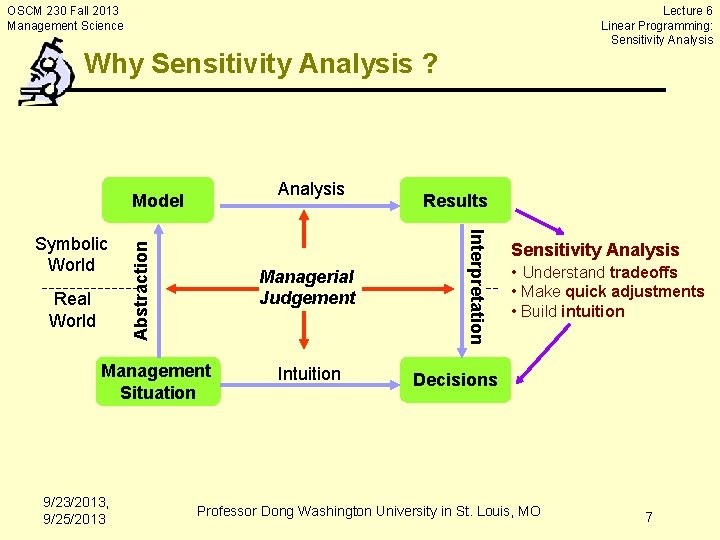
Lecture 6 Linear Programming: Sensitivity Analysis OSCM 230 Fall 2013 Management Science Why Sensitivity Analysis ? Analysis Real World Managerial Judgement Management Situation 9/23/2013, 9/25/2013 Intuition Results Interpretation Symbolic World Abstraction Model Sensitivity Analysis • Understand tradeoffs • Make quick adjustments • Build intuition Decisions Professor Dong Washington University in St. Louis, MO 7

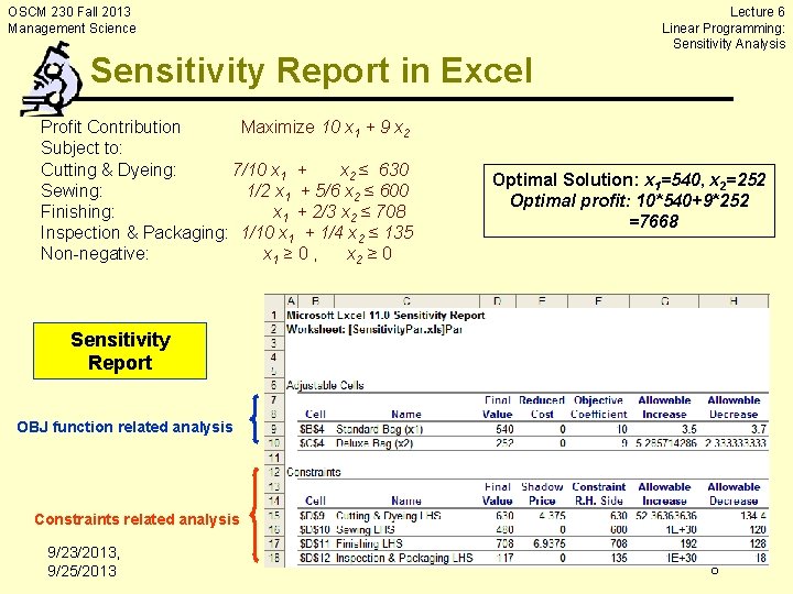
OSCM 230 Fall 2013 Management Science Sensitivity Report in Excel Profit Contribution Maximize 10 x 1 + 9 x 2 Subject to: Cutting & Dyeing: 7/10 x 1 + x 2 ≤ 630 Sewing: 1/2 x 1 + 5/6 x 2 ≤ 600 Finishing: x 1 + 2/3 x 2 ≤ 708 Inspection & Packaging: 1/10 x 1 + 1/4 x 2 ≤ 135 Non-negative: x 1 ≥ 0 , x 2 ≥ 0 Lecture 6 Linear Programming: Sensitivity Analysis Optimal Solution: x 1=540, x 2=252 Optimal profit: 10*540+9*252 =7668 Sensitivity Report OBJ function related analysis Constraints related analysis 9/23/2013, 9/25/2013 8

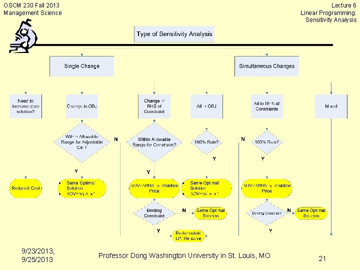
Lecture 6 Linear Programming: Sensitivity Analysis OSCM 230 Fall 2013 Management Science Agenda • Example: Par Inc – Objective function: Change in coefficient • “allowable increase” and “allowable decrease” • “reduced cost” – Constraints: Change in right-hand-side constants • “shadow price” • “allowable increase” and “allowable decrease” – Simultaneous changes • “ 100% rule” • Summary 9/23/2013, 9/25/2013 Professor Dong Washington University in St. Louis, MO 9

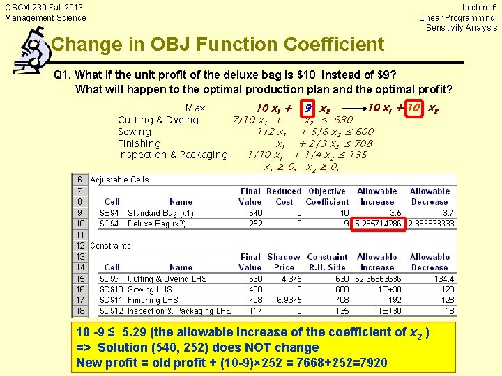
Lecture 6 Linear Programming: Sensitivity Analysis OSCM 230 Fall 2013 Management Science Change in OBJ Function Coefficient Q 1. What if the unit profit of the deluxe bag is $10 instead of $9? What will happen to the optimal production plan and the optimal profit? 10 x 1 + 10 x 2 Max 10 x 1 + 9 x 2 Cutting & Dyeing 7/10 x 1 + x 2 ≤ 630 Sewing 1/2 x 1 + 5/6 x 2 ≤ 600 Finishing x 1 + 2/3 x 2 ≤ 708 Inspection & Packaging 1/10 x 1 + 1/4 x 2 ≤ 135 x 1 ≥ 0, x 2 ≥ 0, 10 -9 ≤ 5. 29 (the allowable increase of the coefficient of x 2 ) => Solution (540, 252) does NOT change New profit = old profit + (10 -9)× 252 = 7668+252=7920 10

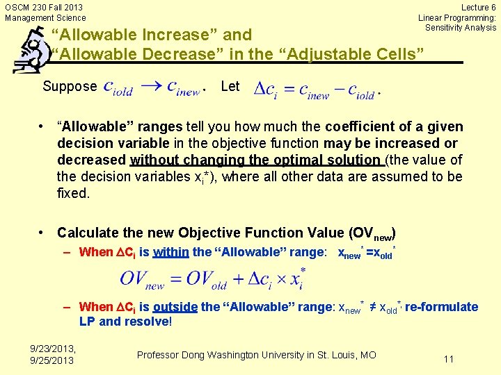
Lecture 6 Linear Programming: Sensitivity Analysis OSCM 230 Fall 2013 Management Science “Allowable Increase” and “Allowable Decrease” in the “Adjustable Cells” Suppose Let • “Allowable” ranges tell you how much the coefficient of a given decision variable in the objective function may be increased or decreased without changing the optimal solution (the value of the decision variables xi*), where all other data are assumed to be fixed. • Calculate the new Objective Function Value (OVnew) – When Ci is within the “Allowable” range: xnew* =xold* – When Ci is outside the “Allowable” range: xnew* ≠ xold*, re-formulate LP and resolve! 9/23/2013, 9/25/2013 Professor Dong Washington University in St. Louis, MO 11

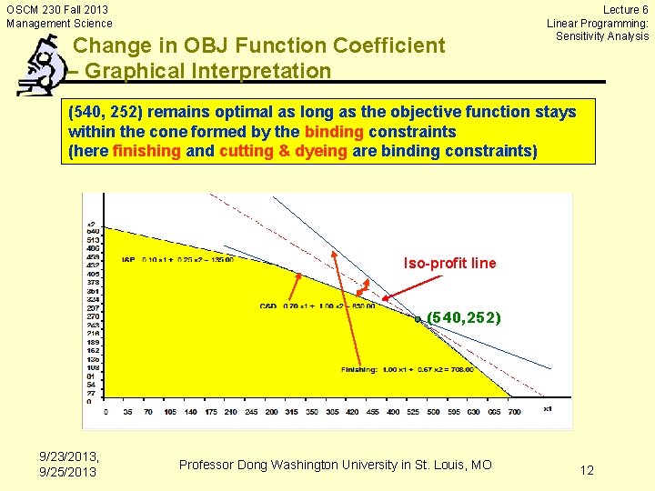
OSCM 230 Fall 2013 Management Science Change in OBJ Function Coefficient – Graphical Interpretation Lecture 6 Linear Programming: Sensitivity Analysis (540, 252) remains optimal as long as the objective function stays within the cone formed by the binding constraints (here finishing and cutting & dyeing are binding constraints) Iso-profit line (540, 252) 9/23/2013, 9/25/2013 Professor Dong Washington University in St. Louis, MO 12

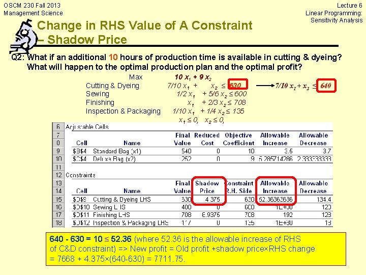
OSCM 230 Fall 2013 Management Science Change in RHS Value of A Constraint – Shadow Price Lecture 6 Linear Programming: Sensitivity Analysis Q 2: What if an additional 10 hours of production time is available in cutting & dyeing? What will happen to the optimal production plan and the optimal profit? Max 10 x 1 + 9 x 2 Cutting & Dyeing 7/10 x 1 + x 2 ≤ 630 Sewing 1/2 x 1 + 5/6 x 2 ≤ 600 Finishing x 1 + 2/3 x 2 ≤ 708 Inspection & Packaging 1/10 x 1 + 1/4 x 2 ≤ 135 x 1 ≤ 0, x 2 ≤ 0, 7/10 x 1 + x 2 ≤ 640 - 630 = 10 ≤ 52. 36 (where 52. 36 is the allowable increase of RHS of C&D constraint) => New profit = Old profit +shadow price×RHS change = 7668 + 4. 375×(640 -630) = 7711. 75. 13

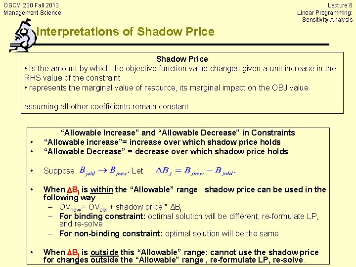
Lecture 6 Linear Programming: Sensitivity Analysis OSCM 230 Fall 2013 Management Science Interpretations of Shadow Price • Is the amount by which the objective function value changes given a unit increase in the RHS value of the constraint • represents the marginal value of resource, its marginal impact on the OBJ value assuming all other coefficients remain constant • • “Allowable Increase” and “Allowable Decrease” in Constraints “Allowable increase”= increase over which shadow price holds “Allowable Decrease” = decrease over which shadow price holds • Suppose • When Bj is within the “Allowable” range : shadow price can be used in the following way – OVnew = OVold + shadow price * ΔBj – For binding constraint: optimal solution will be different, re-formulate LP, and re-solve – For non-binding constraint: optimal solution will be the same. • When Bj is outside this “Allowable” range: cannot use the shadow price for changes outside the “Allowable” range , re-formulate LP, re-solve. Let

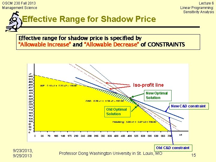
Lecture 6 Linear Programming: Sensitivity Analysis OSCM 230 Fall 2013 Management Science Effective Range for Shadow Price Effective range for shadow price is specified by “Allowable Increase” and “Allowable Decrease” of CONSTRAINTS Iso-profit line New Optimal Solution New C&D constraint Old Optimal Solution 9/23/2013, 9/25/2013 Old C&D constraint Professor Dong Washington University in St. Louis, MO 15

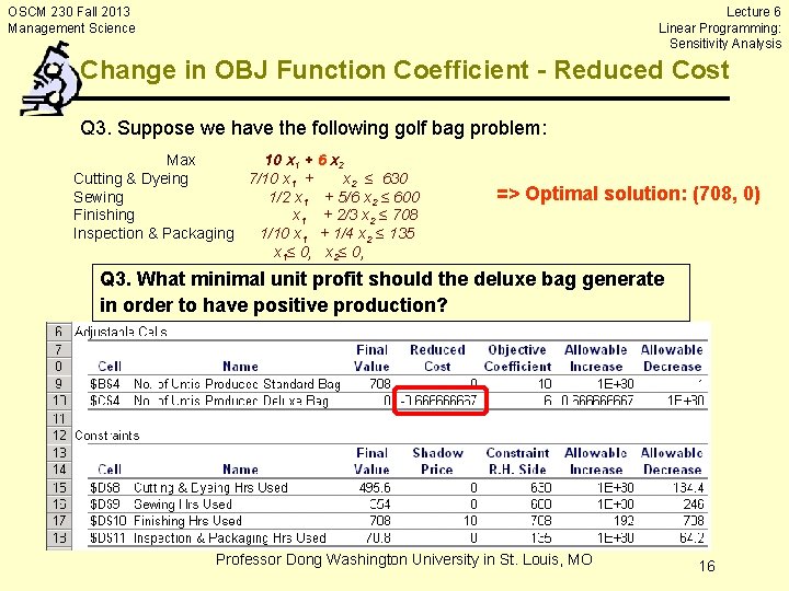
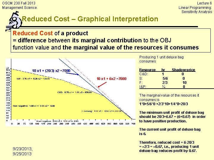
Lecture 6 Linear Programming: Sensitivity Analysis OSCM 230 Fall 2013 Management Science Change in OBJ Function Coefficient - Reduced Cost Q 3. Suppose we have the following golf bag problem: Max 10 x 1 + 6 x 2 Cutting & Dyeing 7/10 x 1 + x 2 ≤ 630 Sewing 1/2 x 1 + 5/6 x 2 ≤ 600 Finishing x 1 + 2/3 x 2 ≤ 708 Inspection & Packaging 1/10 x 1 + 1/4 x 2 ≤ 135 x 1≤ 0, x 2≤ 0, => Optimal solution: (708, 0) Q 3. What minimal unit profit should the deluxe bag generate in order to have positive production? Professor Dong Washington University in St. Louis, MO 16

Lecture 6 Linear Programming: Sensitivity Analysis OSCM 230 Fall 2013 Management Science Reduced Cost – Graphical Interpretation Reduced Cost of a product = difference between its marginal contribution to the OBJ function value and the marginal value of the resources it consumes Producing 1 unit deluxe bag consumes 10 x 1 + (20/3) x 2 =7080 10 x 1 + 6 x 2 =7080 Resource C&D: S: F: I&P: hr 1 5/6 2/3 ¼ Shadow price 0 0 10 0_______ The marginal value of the resources it consumes is 1*0+5/6*0 +2/3*10+1/4*0=20/3 The minimum unit profit of deluxe bag should be 20/3=6. 67 = (6+0. 67) in order to have positive production. The current unit profit of deluxe bag is 6. 9/23/2013, 9/25/2013 Therefore, reduced cost = 6 -20/3 = 2/3 = 0. 67, i. e. , producing 1 unit deluxe bag reduces profit by 0. 67.

OSCM 230 Fall 2013 Management Science Simultaneous Changes in Parameters Lecture 6 Linear Programming: Sensitivity Analysis 1. If all changes are in the objective function coefficients, then you can use the 100% rule. 2. If all changes are in the RHS values, then you can use the 100% rule. 3. If changes are in both the objective function and RHS, you must reformulate and re-solve! 4. If unsure, reformulate and re-solve! 9/23/2013, 9/25/2013 Professor Dong Washington University in St. Louis, MO 18

OSCM 230 Fall 2013 Management Science 100% Rule Lecture 6 Linear Programming: Sensitivity Analysis 1. For all changes that are made, sum the percentages of increase-changes with respect to (w. r. t. ) the corresponding “Allowable Increases” and the percentages of decreasechanges w. r. t. the corresponding “Allowable Decreases, ” in absolute values. 2. For simultaneous OBJ coefficient changes, if the sum of the percentage changes does not exceed 100%, the optimal solution will not change. 3. For simultaneous RHS changes, if the sum of the percentage changes does not exceed 100%, the shadow prices apply. 4. If the sum of the percentage changes DOES exceed 100%, then reformulate and re-solve! 9/23/2013, 9/25/2013 Professor Dong Washington University in St. Louis, MO 19

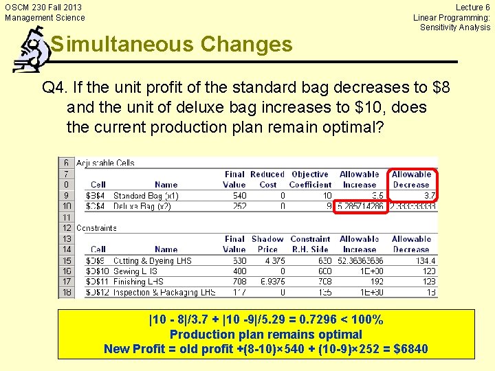
OSCM 230 Fall 2013 Management Science Simultaneous Changes Lecture 6 Linear Programming: Sensitivity Analysis Q 4. If the unit profit of the standard bag decreases to $8 and the unit of deluxe bag increases to $10, does the current production plan remain optimal? |10 - 8|/3. 7 + |10 -9|/5. 29 = 0. 7296 < 100% Production plan remains optimal New Profit = old profit +(8 -10)× 540 + (10 -9)× 252 = $6840 20

Lecture 6 Linear Programming: Sensitivity Analysis OSCM 230 Fall 2013 Management Science 9/23/2013, 9/25/2013 Professor Dong Washington University in St. Louis, MO 21