OSCM 230 Fall 2013 Management Science Lecture 4

OSCM 230 Fall 2013 Management Science Lecture 4 Linear Programming II 9/11/2013, 9/16/2013 Professor Dong Washington University, St. Louis, MO 1

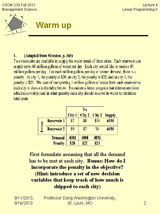
OSCM 230 Fall 2013 Management Science Lecture 4 Linear Programming II Warm up First formulate assuming that all the demand has to be met at each city. Bonus: How do I incorporate the penalty in the objective? (Hint: introduce a set of new decision variables that keep track of how much is shipped to each city) 9/11/2013, 9/16/2013 Professor Dong Washington University, St. Louis, MO 2

OSCM 230 Fall 2013 Management Science Lecture 4 Linear Programming II Agenda • Graphical LP solution • “Special cases” of LP solutions – Infeasible – Multiple optimal solutions – Unbounded • LP formulation guidelines • Formulation examples – Work scheduling – Blending II – RV problem (product mix) 9/11/2013, 9/16/2013 Professor Dong Washington University, St. Louis, MO 3

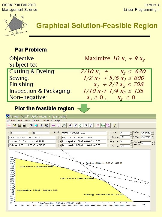
OSCM 230 Fall 2013 Management Science Lecture 4 Linear Programming II Graphical Solution-Feasible Region Par Problem Objective Subject to: Cutting & Dyeing: Sewing: Finishing: Inspection & Packaging: Non-negative: Maximize 10 x 1 + 9 x 2 7/10 x 1 + x 2 ≤ 630 1/2 x 1 + 5/6 x 2 ≤ 600 x 1 + 2/3 x 2 ≤ 708 1/10 x 1+ 1/4 x 2 ≤ 135 x 1 ≥ 0 , x 2 ≥ 0 Plot the feasible region 4

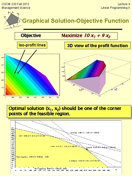
OSCM 230 Fall 2013 Management Science Lecture 4 Linear Programming II Graphical Solution-Objective Function Objective Iso-profit lines Maximize 10 x 1 + 9 x 2 3 D view of the profit function Optimal solution (x 1, x 2) should be one of the corner points of the feasible region. 5

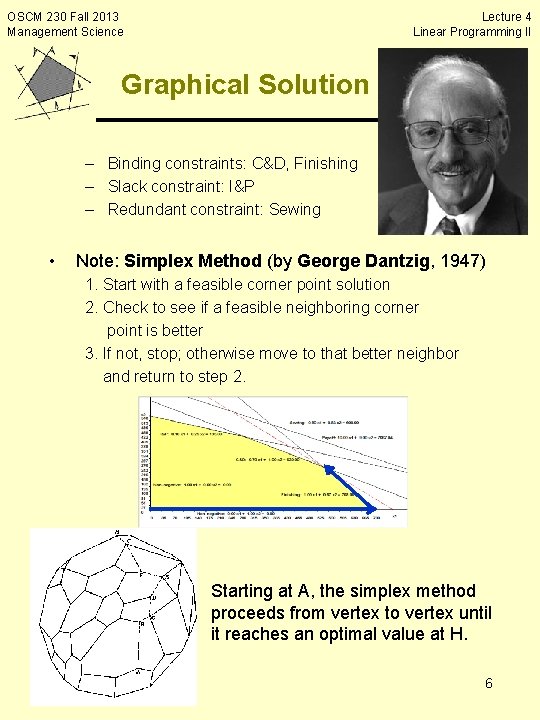
OSCM 230 Fall 2013 Management Science Lecture 4 Linear Programming II Graphical Solution – Cont’d – Binding constraints: C&D, Finishing – Slack constraint: I&P – Redundant constraint: Sewing • Note: Simplex Method (by George Dantzig, 1947) 1. Start with a feasible corner point solution 2. Check to see if a feasible neighboring corner point is better 3. If not, stop; otherwise move to that better neighbor and return to step 2. Starting at A, the simplex method proceeds from vertex to vertex until it reaches an optimal value at H. 9/11/2013, 9/16/2013 6

OSCM 230 Fall 2013 Management Science Lecture 4 Linear Programming II Product Mix Example Par, Inc. Problem Par, Inc. manufactures two types of golf bags: standard and deluxe. The profit contribution of a standard golf bag is $10. The profit contribution of a deluxe golf bag is $9. The production of golf bags mainly consists of four steps: cutting & dyeing, sewing, finishing, inspection & packaging. Each standard golf bag requires 7/10 hours of cutting& dyeing, 1/2 hour of sewing, 1 hour of finishing, and 0. 1 hour of inspection & packaging. Each deluxe golf bag requires 1 hours of cutting & dyeing, 5/6 hour of sewing, 2/3 hour of finishing, and 1/4 hour of inspection & packaging. Demand for golf bags is unlimited. However, due to the capacity and labor constraints, each week Par has at most 630 hours of cutting & dyeing, 600 hours of sewing, 708 hours of finishing, and 135 hours of inspection and packaging for the production of golf bags. Par wishes to maximize weekly profit. Formulate a mathematical model of Par's situation that can be used to maximize weekly profit. Professor Dong Washington University, St. 9/9/2013 7

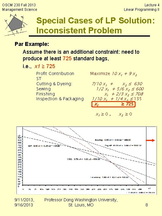
OSCM 230 Fall 2013 Management Science Lecture 4 Linear Programming II Special Cases of LP Solution: Inconsistent Problem Par Example: Assume there is an additional constraint: need to produce at least 725 standard bags, i. e. , x 1 ≥ 725 Profit Contribution ST Cutting & Dyeing: Sewing Finishing Inspection & Packaging Maximize 10 x 1 + 9 x 2 7/10 x 1 + x 2 ≤ 630 1/2 x 1 + 5/6 x 2 ≤ 600 x 1 + 2/3 x 2 ≤ 708 1/10 x 1 + 1/4 x 2 ≤ 135 x 1 ≥ 725 x 1 ≥ 0 , 9/11/2013, 9/16/2013 Professor Dong Washington University, St. Louis, MO x 2 ≥ 0 8

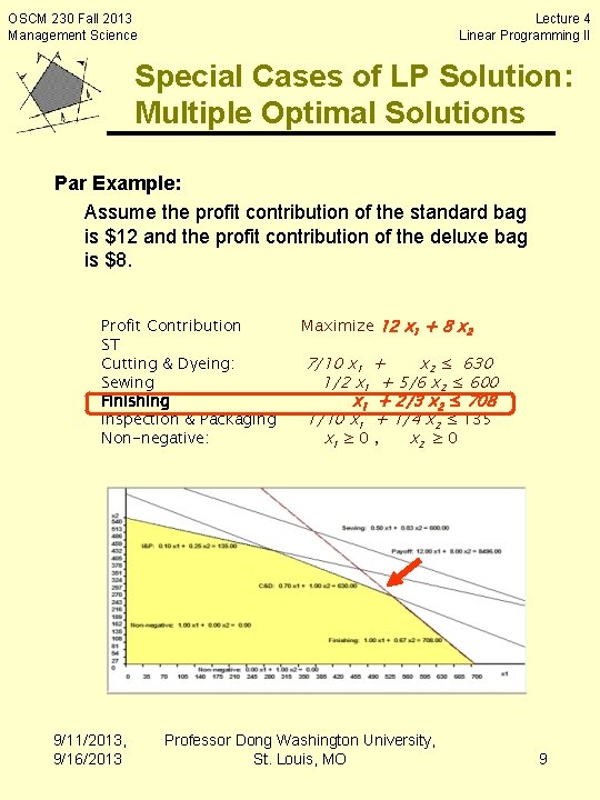
OSCM 230 Fall 2013 Management Science Lecture 4 Linear Programming II Special Cases of LP Solution: Multiple Optimal Solutions Par Example: Assume the profit contribution of the standard bag is $12 and the profit contribution of the deluxe bag is $8. Profit Contribution ST Cutting & Dyeing: Sewing Finishing Inspection & Packaging Non-negative: 9/11/2013, 9/16/2013 Maximize 12 x 1 + 8 x 2 7/10 x 1 + x 2 ≤ 630 1/2 x 1 + 5/6 x 2 ≤ 600 x 1 + 2/3 x 2 ≤ 708 1/10 x 1 + 1/4 x 2 ≤ 135 x 1 ≥ 0 , x 2 ≥ 0 Professor Dong Washington University, St. Louis, MO 9

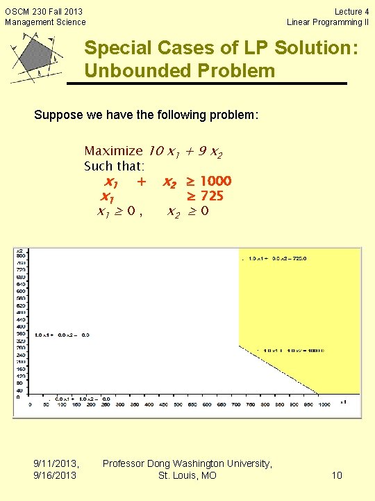
OSCM 230 Fall 2013 Management Science Lecture 4 Linear Programming II Special Cases of LP Solution: Unbounded Problem Suppose we have the following problem: Maximize 10 x 1 + 9 x 2 Such that: x 1 + x 2 ≥ 1000 x 1 ≥ 725 x 1 ≥ 0 , x 2 ≥ 0 9/11/2013, 9/16/2013 Professor Dong Washington University, St. Louis, MO 10

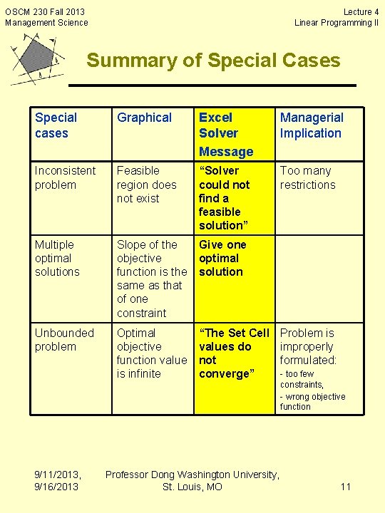
OSCM 230 Fall 2013 Management Science Lecture 4 Linear Programming II Summary of Special Cases Special cases Graphical Excel Solver Message Managerial Implication Inconsistent problem Feasible region does not exist “Solver could not find a feasible solution” Too many restrictions Multiple optimal solutions Slope of the objective function is the same as that of one constraint Give one optimal solution Unbounded problem Optimal objective function value is infinite “The Set Cell Problem is values do improperly not formulated: - too few converge” 9/11/2013, 9/16/2013 Professor Dong Washington University, St. Louis, MO constraints, - wrong objective function 11

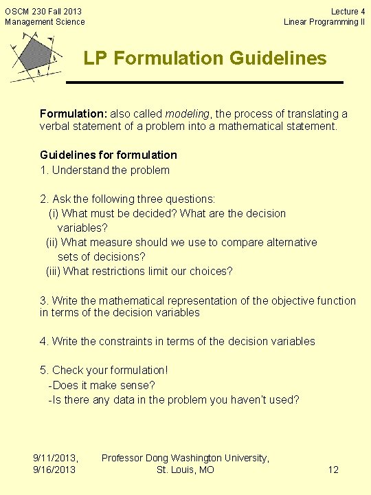
OSCM 230 Fall 2013 Management Science Lecture 4 Linear Programming II LP Formulation Guidelines Formulation: also called modeling, the process of translating a verbal statement of a problem into a mathematical statement. Guidelines formulation 1. Understand the problem 2. Ask the following three questions: (i) What must be decided? What are the decision variables? (ii) What measure should we use to compare alternative sets of decisions? (iii) What restrictions limit our choices? 3. Write the mathematical representation of the objective function in terms of the decision variables 4. Write the constraints in terms of the decision variables 5. Check your formulation! -Does it make sense? -Is there any data in the problem you haven’t used? 9/11/2013, 9/16/2013 Professor Dong Washington University, St. Louis, MO 12

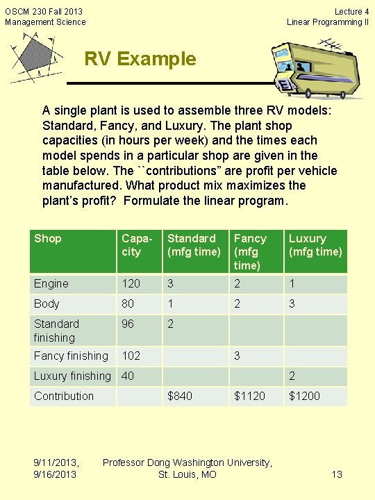
OSCM 230 Fall 2013 Management Science Lecture 4 Linear Programming II RV Example A single plant is used to assemble three RV models: Standard, Fancy, and Luxury. The plant shop capacities (in hours per week) and the times each model spends in a particular shop are given in the table below. The ``contributions” are profit per vehicle manufactured. What product mix maximizes the plant’s profit? Formulate the linear program. Shop Capacity Standard (mfg time) Fancy (mfg time) Luxury (mfg time) Engine 120 3 2 1 Body 80 1 2 3 Standard finishing 96 2 Fancy finishing 102 3 Luxury finishing 40 Contribution 9/11/2013, 9/16/2013 2 $840 $1120 Professor Dong Washington University, St. Louis, MO $1200 13

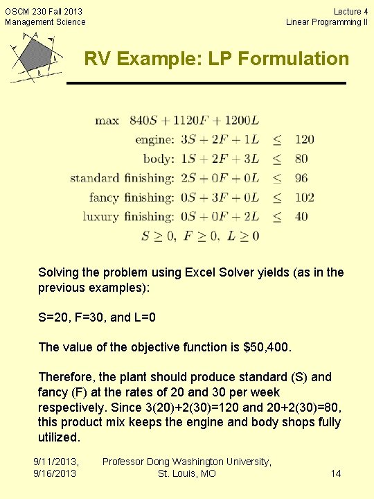
OSCM 230 Fall 2013 Management Science Lecture 4 Linear Programming II RV Example: LP Formulation Solving the problem using Excel Solver yields (as in the previous examples): S=20, F=30, and L=0 The value of the objective function is $50, 400. Therefore, the plant should produce standard (S) and fancy (F) at the rates of 20 and 30 per week respectively. Since 3(20)+2(30)=120 and 20+2(30)=80, this product mix keeps the engine and body shops fully utilized. 9/11/2013, 9/16/2013 Professor Dong Washington University, St. Louis, MO 14

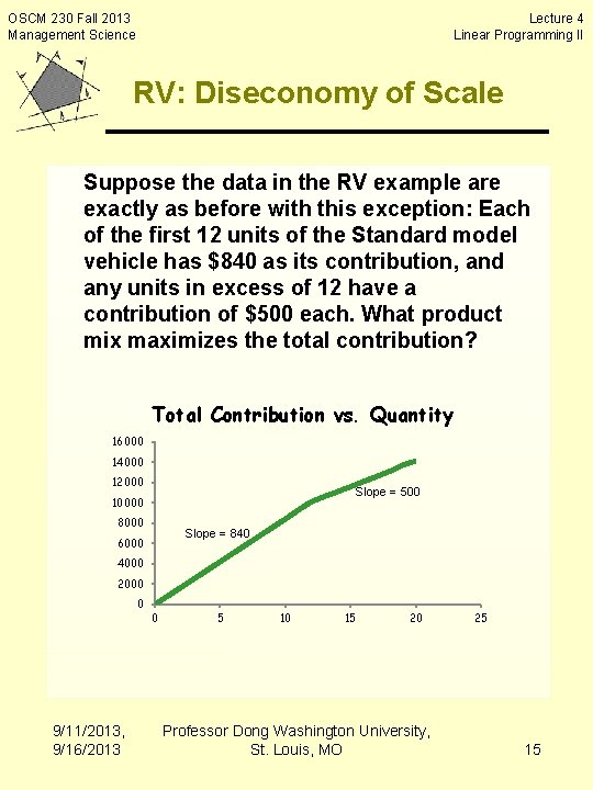
OSCM 230 Fall 2013 Management Science Lecture 4 Linear Programming II RV: Diseconomy of Scale Suppose the data in the RV example are exactly as before with this exception: Each of the first 12 units of the Standard model vehicle has $840 as its contribution, and any units in excess of 12 have a contribution of $500 each. What product mix maximizes the total contribution? Total Contribution vs. Quantity 16000 14000 12000 Slope = 500 10000 8000 Slope = 840 6000 4000 2000 0 9/11/2013, 9/16/2013 0 5 10 15 20 Professor Dong Washington University, St. Louis, MO 25 15

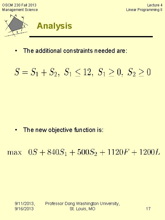
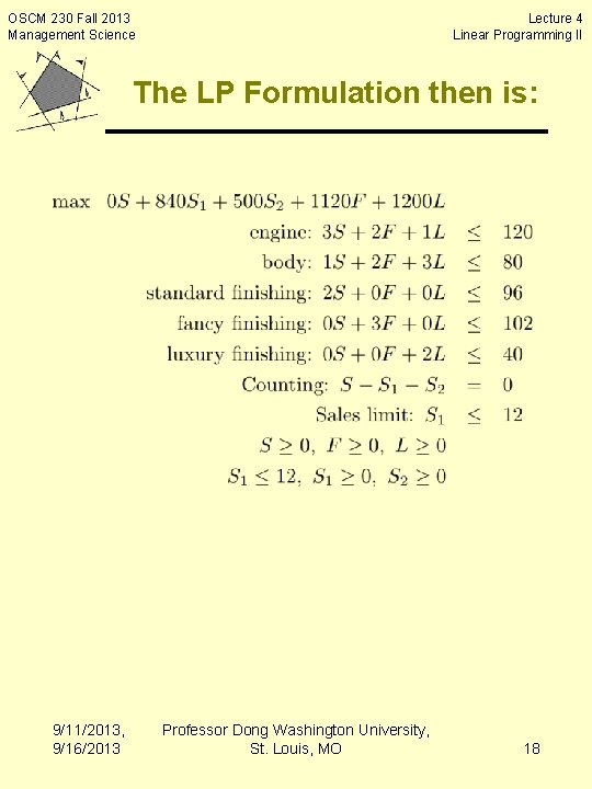
OSCM 230 Fall 2013 Management Science Lecture 4 Linear Programming II Analysis • The model has become less profitable so we may anticipate to make fewer of them • However, it is not clear that we make fewer than twelve at $840 apiece • To re-solve this problem, we need to change the previous linear program in three ways. The first change is to introduce two new decision variables – S 1 = the number of Standard model vehicles made per week and sold a contribution of $840 each – S 2 = the number of Standard model vehicles made per week and sold a contribution of $500 each • The second and third change add constraints and change the objective function 9/11/2013, 9/16/2013 Professor Dong Washington University, St. Louis, MO 16

OSCM 230 Fall 2013 Management Science Lecture 4 Linear Programming II Analysis • The additional constraints needed are: • The new objective function is: 9/11/2013, 9/16/2013 Professor Dong Washington University, St. Louis, MO 17

OSCM 230 Fall 2013 Management Science Lecture 4 Linear Programming II The LP Formulation then is: 9/11/2013, 9/16/2013 Professor Dong Washington University, St. Louis, MO 18

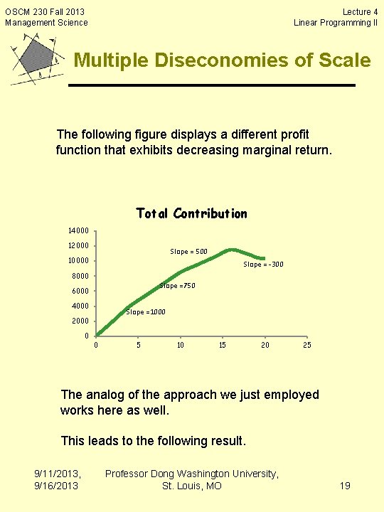
OSCM 230 Fall 2013 Management Science Lecture 4 Linear Programming II Multiple Diseconomies of Scale The following figure displays a different profit function that exhibits decreasing marginal return. Total Contribution 14000 12000 Slope = 500 10000 Slope = -300 8000 Slope =750 6000 4000 Slope =1000 2000 0 0 5 10 15 20 25 The analog of the approach we just employed works here as well. This leads to the following result. 9/11/2013, 9/16/2013 Professor Dong Washington University, St. Louis, MO 19

OSCM 230 Fall 2013 Management Science Lecture 4 Linear Programming II Multiple Diseconomies of Scale A linear program readily accommodates decreasing marginal return, increasing marginal cost, and other diseconomies of scale. Summary 1. Intuition behind the Simplex algorithm 2. Additional LP formulations 3. Accommodations of piece-wise linearity 9/11/2013, 9/16/2013 Professor Dong Washington University, St. Louis, MO 20