Lecture 3 PAC Learning VC Dimension and Mistake

Lecture 3 PAC Learning, VC Dimension, and Mistake Bounds Thursday, September 2, 1999 William H. Hsu Department of Computing and Information Sciences, KSU http: //www. cis. ksu. edu/~bhsu Readings: Sections 7. 4. 1 -7. 4. 3, 7. 5. 1 -7. 5. 3, Mitchell Chapter 1, Kearns and Vazirani CIS 798: Intelligent Systems and Machine Learning Kansas State University Department of Computing and Information Sciences

Lecture Outline • Read 7. 4. 1 -7. 4. 3, 7. 5. 1 -7. 5. 3, Mitchell; Chapter 1, Kearns and Vazirani • Suggested Exercises: 7. 2, Mitchell; 1. 1, Kearns and Vazirani • PAC Learning (Continued) – Examples and results: learning rectangles, normal forms, conjunctions – What PAC analysis reveals about problem difficulty – Turning PAC results into design choices • Occam’s Razor: A Formal Inductive Bias – Preference for shorter hypotheses – More on Occam’s Razor when we get to decision trees • Vapnik-Chervonenkis (VC) Dimension – Objective: label any instance of (shatter) a set of points with a set of functions – VC(H): a measure of the expressiveness of hypothesis space H • Mistake Bounds – Estimating the number of mistakes made before convergence – Optimal error bounds CIS 798: Intelligent Systems and Machine Learning Kansas State University Department of Computing and Information Sciences

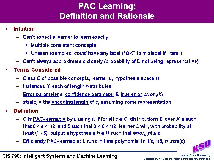
PAC Learning: Definition and Rationale • Intuition – Can’t expect a learner to learn exactly • Multiple consistent concepts • Unseen examples: could have any label (“OK” to mislabel if “rare”) – Can’t always approximate c closely (probability of D not being representative) • Terms Considered – Class C of possible concepts, learner L, hypothesis space H – Instances X, each of length n attributes – Error parameter , confidence parameter , true error. D(h) – size(c) = the encoding length of c, assuming some representation • Definition – C is PAC-learnable by L using H if for all c C, distributions D over X, such that 0 < < 1/2, and such that 0 < < 1/2, learner L will, with probability at least (1 - ), output a hypothesis h H such that error. D(h) – Efficiently PAC-learnable: L runs in time polynomial in 1/ , n, size(c) CIS 798: Intelligent Systems and Machine Learning Kansas State University Department of Computing and Information Sciences

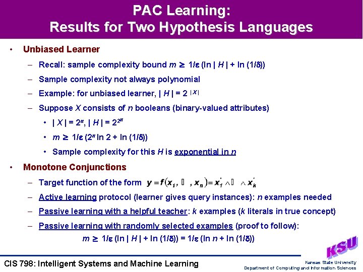
PAC Learning: Results for Two Hypothesis Languages • Unbiased Learner – Recall: sample complexity bound m 1/ (ln | H | + ln (1/ )) – Sample complexity not always polynomial – Example: for unbiased learner, | H | = 2 | X | – Suppose X consists of n booleans (binary-valued attributes) • | X | = 2 n , | H | = 2 2 n • m 1/ (2 n ln 2 + ln (1/ )) • Sample complexity for this H is exponential in n • Monotone Conjunctions – Target function of the form – Active learning protocol (learner gives query instances): n examples needed – Passive learning with a helpful teacher: k examples (k literals in true concept) – Passive learning with randomly selected examples (proof to follow): m 1/ (ln | H | + ln (1/ )) = 1/ (ln n + ln (1/ )) CIS 798: Intelligent Systems and Machine Learning Kansas State University Department of Computing and Information Sciences

PAC Learning: Monotone Conjunctions [1] • Monotone Conjunctive Concepts – Suppose c C (and h H) is of the form x 1 x 2 … xm – n possible variables: either omitted or included (i. e. , positive literals only) • Errors of Omission (False Negatives) – Claim: the only possible errors are false negatives (h(x) = -, c(x) = +) – Mistake iff (z h) (z c) ( x Dtest. x(z) = false): then h(x) = -, c(x) = + • Probability of False Negatives – Let z be a literal; let Pr(Z) be the probability that z is false in a positive x D – z in target concept (correct conjunction c = x 1 x 2 … xm) Pr(Z) = 0 – Pr(Z) is the probability that a randomly chosen positive example has z = false (inducing a potential mistake, or deleting z from h if training is still in progress) Instance Space X – error(h) z h Pr(Z) - c - CIS 798: Intelligent Systems and Machine Learning h + + + - Kansas State University Department of Computing and Information Sciences

PAC Learning: Monotone Conjunctions [2] • Bad Literals – Call a literal z bad if Pr(Z) > = ’/n – z does not belong in h, and is likely to be dropped (by appearing with value true in a positive x D), but has not yet appeared in such an example • Case of No Bad Literals – Lemma: if there are no bad literals, then error(h) ’ – Proof: error(h) z h Pr(Z) z h ’/n ’ (worst case: all n z’s are in c ~ h) • Case of Some Bad Literals – Let z be a bad literal – Survival probability (probability that it will not be eliminated by a given example): 1 - Pr(Z) < 1 - ’/n – Survival probability over m examples: (1 - Pr(Z))m < (1 - ’/n)m – Worst case survival probability over m examples (n bad literals) = n (1 - ’/n)m – Intuition: more chance of a mistake = greater chance to learn CIS 798: Intelligent Systems and Machine Learning Kansas State University Department of Computing and Information Sciences

PAC Learning: Monotone Conjunctions [3] • Goal: Achieve An Upper Bound for Worst-Case Survival Probability – Choose m large enough so that probability of a bad literal z surviving across m examples is less than – Pr(z survives m examples) = n (1 - ’/n)m < – Solve for m using inequality 1 - x < e-x • n e-m ’/n < • m > n/ ’ (ln (n) + ln (1/ )) examples needed to guarantee the bounds – This completes the proof of the PAC result for monotone conjunctions – Nota Bene: a specialization of m 1/ (ln | H | + ln (1/ )); n/ ’ = 1/ • Practical Ramifications – Suppose = 0. 1, ’ = 0. 1, n = 100: we need 6907 examples – Suppose = 0. 1, ’ = 0. 1, n = 10: we need only 460 examples – Suppose = 0. 01, ’ = 0. 1, n = 10: we need only 690 examples CIS 798: Intelligent Systems and Machine Learning Kansas State University Department of Computing and Information Sciences

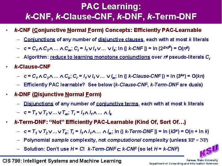
PAC Learning: k-CNF, k-Clause-CNF, k-DNF, k-Term-DNF • k-CNF (Conjunctive Normal Form) Concepts: Efficiently PAC-Learnable – Conjunctions of any number of disjunctive clauses, each with at most k literals – c = C 1 C 2 … Cm; Ci = l 1 … lk; ln (| k-CNF |) = ln (2(2 n)k) = (nk) – Algorithm: reduce to learning monotone conjunctions over nk pseudo-literals Ci • k-Clause-CNF – c = C 1 C 2 … Ck; Ci = l 1 … lm; ln (| k-Clause-CNF |) = ln (3 kn) = (kn) – Efficiently PAC learnable? See below (k-Clause-CNF, k-Term-DNF are duals) • k-DNF (Disjunctive Normal Form) – Disjunctions of any number of conjunctive terms, each with at most k literals – c = T 1 T 2 … Tm; Ti = l 1 … lk • k-Term-DNF: “Not” Efficiently PAC-Learnable (Kind Of, Sort Of…) – c = T 1 T 2 … Tk; Ti = l 1 … lm; ln (| k-Term-DNF |) = ln (k 3 n) = (n + ln k) – Polynomial sample complexity, not computational complexity (unless RP = NP) – Solution: Don’t use H = C! k-Term-DNF k-CNF (so let H = k-CNF) CIS 798: Intelligent Systems and Machine Learning Kansas State University Department of Computing and Information Sciences

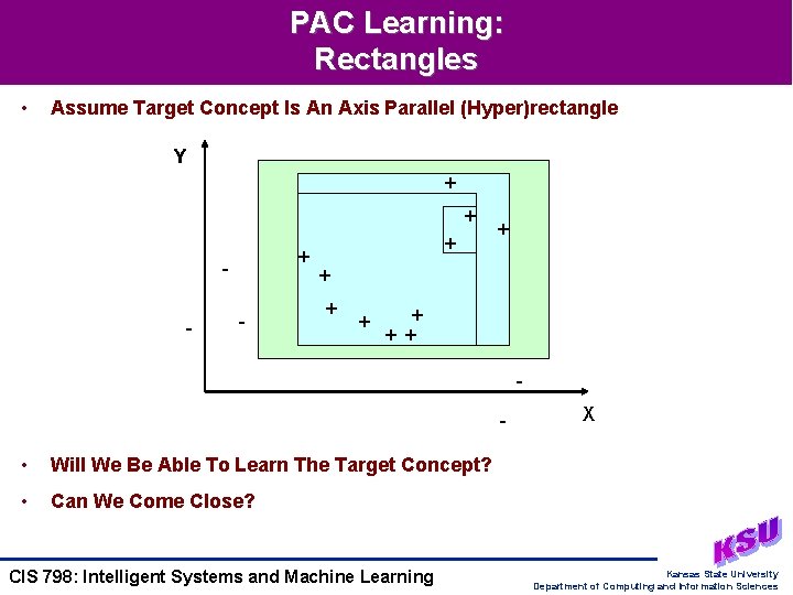
PAC Learning: Rectangles • Assume Target Concept Is An Axis Parallel (Hyper)rectangle Y + + + - - + + + + - • Will We Be Able To Learn The Target Concept? • Can We Come Close? CIS 798: Intelligent Systems and Machine Learning X Kansas State University Department of Computing and Information Sciences

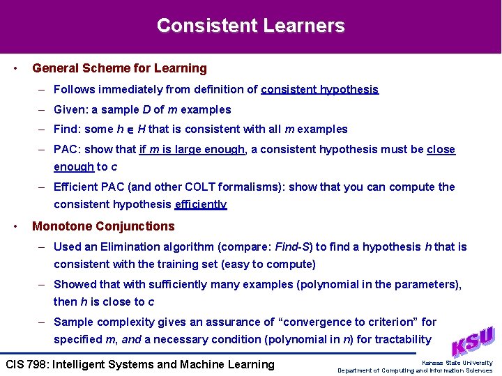
Consistent Learners • General Scheme for Learning – Follows immediately from definition of consistent hypothesis – Given: a sample D of m examples – Find: some h H that is consistent with all m examples – PAC: show that if m is large enough, a consistent hypothesis must be close enough to c – Efficient PAC (and other COLT formalisms): show that you can compute the consistent hypothesis efficiently • Monotone Conjunctions – Used an Elimination algorithm (compare: Find-S) to find a hypothesis h that is consistent with the training set (easy to compute) – Showed that with sufficiently many examples (polynomial in the parameters), then h is close to c – Sample complexity gives an assurance of “convergence to criterion” for specified m, and a necessary condition (polynomial in n) for tractability CIS 798: Intelligent Systems and Machine Learning Kansas State University Department of Computing and Information Sciences

Occam’s Razor and PAC Learning [1] • Bad Hypothesis – – Want to bound: probability that there exists a hypothesis h H that • is consistent with m examples • satisfies error. D(h) > – Claim: the probability is less than | H | (1 - )m • Proof – Let h be such a bad hypothesis – The probability that h is consistent with one example <x, c(x)> of c is – Because the m examples are drawn independently of each other, the probability that h is consistent with m examples of c is less than (1 - )m – The probability that some hypothesis in H is consistent with m examples of c is less than | H | (1 - )m , Quod Erat Demonstrandum CIS 798: Intelligent Systems and Machine Learning Kansas State University Department of Computing and Information Sciences

Occam’s Razor and PAC Learning [2] • Goal – We want this probability to be smaller than , that is: • | H | (1 - )m < • ln (| H |) + m ln (1 - ) < ln ( ) – With ln (1 - ) : m 1/ (ln | H | + ln (1/ )) – This is the result from last time [Blumer et al, 1987; Haussler, 1988] • Occam’s Razor – “Entities should not be multiplied without necessity” – So called because it indicates a preference towards a small H – Why do we want small H? • Generalization capability: explicit form of inductive bias • Search capability: more efficient, compact – To guarantee consistency, need H C – really want the smallest H possible? CIS 798: Intelligent Systems and Machine Learning Kansas State University Department of Computing and Information Sciences

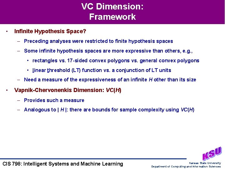
VC Dimension: Framework • Infinite Hypothesis Space? – Preceding analyses were restricted to finite hypothesis spaces – Some infinite hypothesis spaces are more expressive than others, e. g. , • rectangles vs. 17 -sided convex polygons vs. general convex polygons • linear threshold (LT) function vs. a conjunction of LT units – Need a measure of the expressiveness of an infinite H other than its size • Vapnik-Chervonenkis Dimension: VC(H) – Provides such a measure – Analogous to | H |: there are bounds for sample complexity using VC(H) CIS 798: Intelligent Systems and Machine Learning Kansas State University Department of Computing and Information Sciences

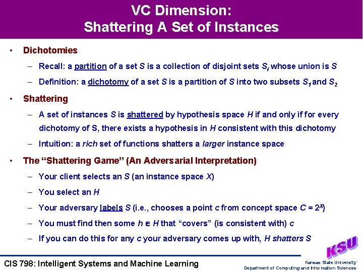
VC Dimension: Shattering A Set of Instances • Dichotomies – Recall: a partition of a set S is a collection of disjoint sets Si whose union is S – Definition: a dichotomy of a set S is a partition of S into two subsets S 1 and S 2 • Shattering – A set of instances S is shattered by hypothesis space H if and only if for every dichotomy of S, there exists a hypothesis in H consistent with this dichotomy – Intuition: a rich set of functions shatters a larger instance space • The “Shattering Game” (An Adversarial Interpretation) – Your client selects an S (an instance space X) – You select an H – Your adversary labels S (i. e. , chooses a point c from concept space C = 2 X) – You must find then some h H that “covers” (is consistent with) c – If you can do this for any c your adversary comes up with, H shatters S CIS 798: Intelligent Systems and Machine Learning Kansas State University Department of Computing and Information Sciences

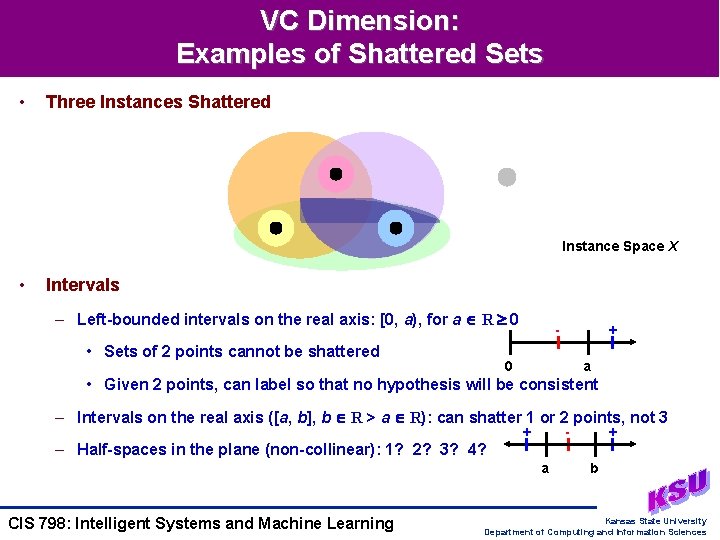
VC Dimension: Examples of Shattered Sets • Three Instances Shattered Instance Space X • Intervals – Left-bounded intervals on the real axis: [0, a), for a R 0 • Sets of 2 points cannot be shattered - + 0 a • Given 2 points, can label so that no hypothesis will be consistent – Intervals on the real axis ([a, b], b R > a R): can shatter 1 or 2 points, not 3 + - + – Half-spaces in the plane (non-collinear): 1? 2? 3? 4? a CIS 798: Intelligent Systems and Machine Learning b Kansas State University Department of Computing and Information Sciences

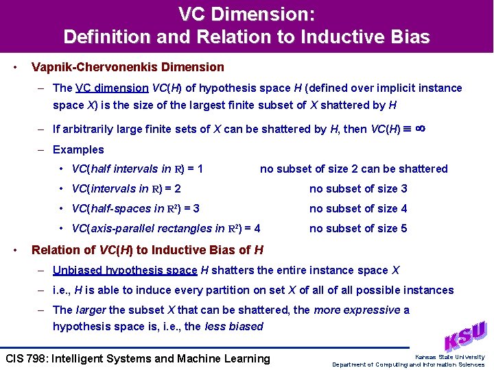
VC Dimension: Definition and Relation to Inductive Bias • Vapnik-Chervonenkis Dimension – The VC dimension VC(H) of hypothesis space H (defined over implicit instance space X) is the size of the largest finite subset of X shattered by H – If arbitrarily large finite sets of X can be shattered by H, then VC(H) – Examples • VC(half intervals in R) = 1 • no subset of size 2 can be shattered • VC(intervals in R) = 2 no subset of size 3 • VC(half-spaces in R 2) = 3 no subset of size 4 • VC(axis-parallel rectangles in R 2) = 4 no subset of size 5 Relation of VC(H) to Inductive Bias of H – Unbiased hypothesis space H shatters the entire instance space X – i. e. , H is able to induce every partition on set X of all possible instances – The larger the subset X that can be shattered, the more expressive a hypothesis space is, i. e. , the less biased CIS 798: Intelligent Systems and Machine Learning Kansas State University Department of Computing and Information Sciences

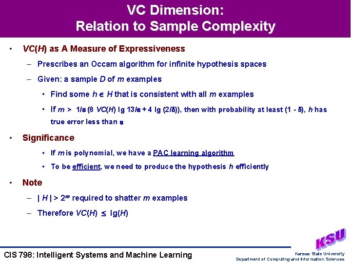
VC Dimension: Relation to Sample Complexity • VC(H) as A Measure of Expressiveness – Prescribes an Occam algorithm for infinite hypothesis spaces – Given: a sample D of m examples • Find some h H that is consistent with all m examples • If m > 1/ (8 VC(H) lg 13/ + 4 lg (2/ )), then with probability at least (1 - ), h has true error less than • Significance • If m is polynomial, we have a PAC learning algorithm • To be efficient, we need to produce the hypothesis h efficiently • Note – | H | > 2 m required to shatter m examples – Therefore VC(H) lg(H) CIS 798: Intelligent Systems and Machine Learning Kansas State University Department of Computing and Information Sciences

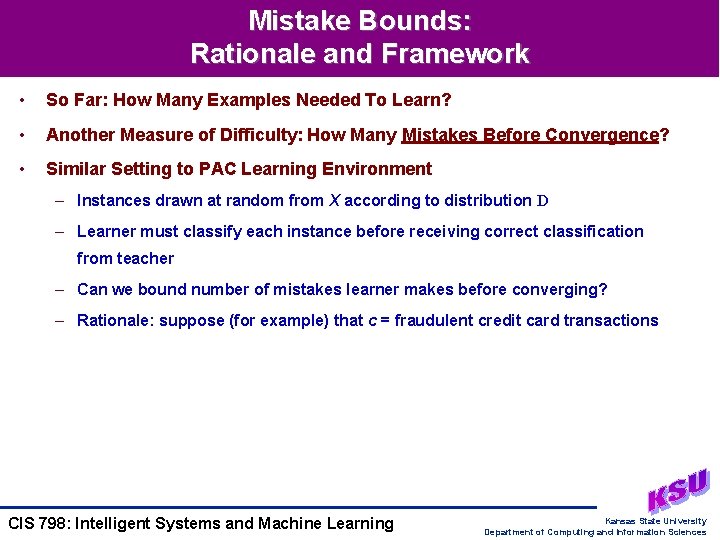
Mistake Bounds: Rationale and Framework • So Far: How Many Examples Needed To Learn? • Another Measure of Difficulty: How Many Mistakes Before Convergence? • Similar Setting to PAC Learning Environment – Instances drawn at random from X according to distribution D – Learner must classify each instance before receiving correct classification from teacher – Can we bound number of mistakes learner makes before converging? – Rationale: suppose (for example) that c = fraudulent credit card transactions CIS 798: Intelligent Systems and Machine Learning Kansas State University Department of Computing and Information Sciences

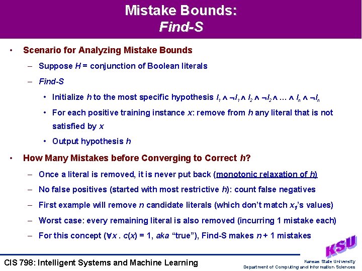
Mistake Bounds: Find-S • Scenario for Analyzing Mistake Bounds – Suppose H = conjunction of Boolean literals – Find-S • Initialize h to the most specific hypothesis l 1 l 2 … ln • For each positive training instance x: remove from h any literal that is not satisfied by x • Output hypothesis h • How Many Mistakes before Converging to Correct h? – Once a literal is removed, it is never put back (monotonic relaxation of h) – No false positives (started with most restrictive h): count false negatives – First example will remove n candidate literals (which don’t match x 1’s values) – Worst case: every remaining literal is also removed (incurring 1 mistake each) – For this concept ( x. c(x) = 1, aka “true”), Find-S makes n + 1 mistakes CIS 798: Intelligent Systems and Machine Learning Kansas State University Department of Computing and Information Sciences

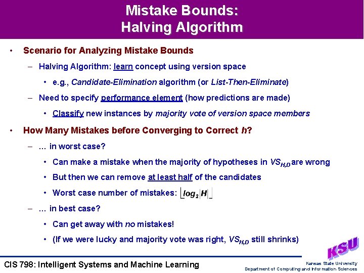
Mistake Bounds: Halving Algorithm • Scenario for Analyzing Mistake Bounds – Halving Algorithm: learn concept using version space • e. g. , Candidate-Elimination algorithm (or List-Then-Eliminate) – Need to specify performance element (how predictions are made) • Classify new instances by majority vote of version space members • How Many Mistakes before Converging to Correct h? – … in worst case? • Can make a mistake when the majority of hypotheses in VSH, D are wrong • But then we can remove at least half of the candidates • Worst case number of mistakes: – … in best case? • Can get away with no mistakes! • (If we were lucky and majority vote was right, VSH, D still shrinks) CIS 798: Intelligent Systems and Machine Learning Kansas State University Department of Computing and Information Sciences

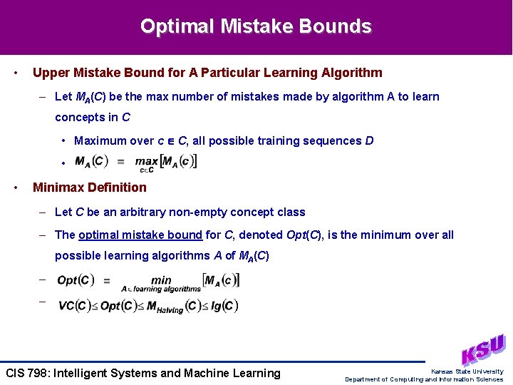
Optimal Mistake Bounds • Upper Mistake Bound for A Particular Learning Algorithm – Let MA(C) be the max number of mistakes made by algorithm A to learn concepts in C • Maximum over c C, all possible training sequences D • • Minimax Definition – Let C be an arbitrary non-empty concept class – The optimal mistake bound for C, denoted Opt(C), is the minimum over all possible learning algorithms A of MA(C) – – CIS 798: Intelligent Systems and Machine Learning Kansas State University Department of Computing and Information Sciences

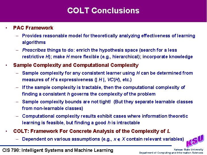
COLT Conclusions • PAC Framework – Provides reasonable model for theoretically analyzing effectiveness of learning algorithms – Prescribes things to do: enrich the hypothesis space (search for a less restrictive H); make H more flexible (e. g. , hierarchical); incorporate knowledge • Sample Complexity and Computational Complexity – Sample complexity for any consistent learner using H can be determined from measures of H’s expressiveness (| H |, VC(H), etc. ) – If the sample complexity is tractable, then the computational complexity of finding a consistent h governs the complexity of the problem – Sample complexity bounds are not tight! (But they separate learnable classes from non-learnable classes) – Computational complexity results exhibit cases where information theoretic learning is feasible, but finding a good h is intractable • COLT: Framework For Concrete Analysis of the Complexity of L – Dependent on various assumptions (e. g. , x X contain relevant variables) CIS 798: Intelligent Systems and Machine Learning Kansas State University Department of Computing and Information Sciences

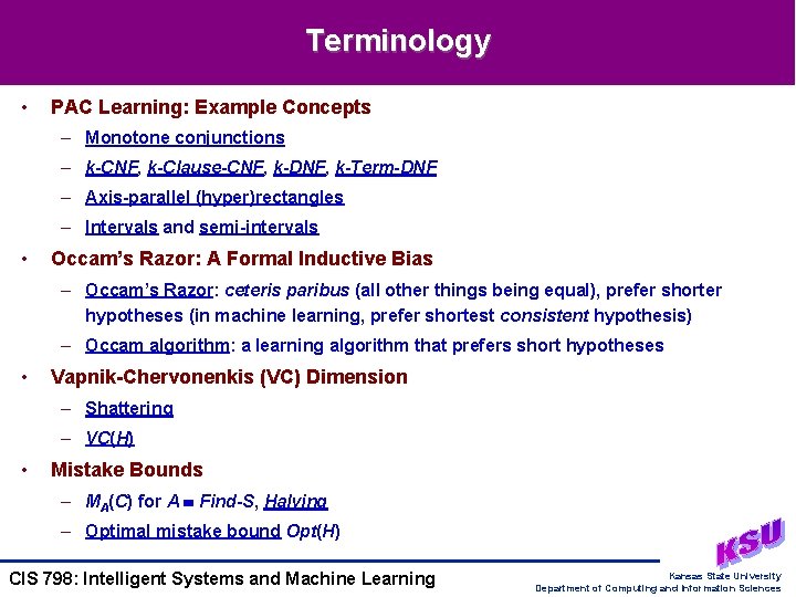
Terminology • PAC Learning: Example Concepts – Monotone conjunctions – k-CNF, k-Clause-CNF, k-DNF, k-Term-DNF – Axis-parallel (hyper)rectangles – Intervals and semi-intervals • Occam’s Razor: A Formal Inductive Bias – Occam’s Razor: ceteris paribus (all other things being equal), prefer shorter hypotheses (in machine learning, prefer shortest consistent hypothesis) – Occam algorithm: a learning algorithm that prefers short hypotheses • Vapnik-Chervonenkis (VC) Dimension – Shattering – VC(H) • Mistake Bounds – MA(C) for A Find-S, Halving – Optimal mistake bound Opt(H) CIS 798: Intelligent Systems and Machine Learning Kansas State University Department of Computing and Information Sciences

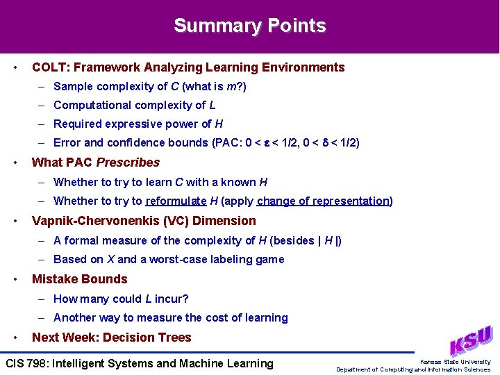
Summary Points • COLT: Framework Analyzing Learning Environments – Sample complexity of C (what is m? ) – Computational complexity of L – Required expressive power of H – Error and confidence bounds (PAC: 0 < < 1/2, 0 < < 1/2) • What PAC Prescribes – Whether to try to learn C with a known H – Whether to try to reformulate H (apply change of representation) • Vapnik-Chervonenkis (VC) Dimension – A formal measure of the complexity of H (besides | H |) – Based on X and a worst-case labeling game • Mistake Bounds – How many could L incur? – Another way to measure the cost of learning • Next Week: Decision Trees CIS 798: Intelligent Systems and Machine Learning Kansas State University Department of Computing and Information Sciences