Lecture 3 Linear random intercept models Example Weight

Lecture 3 Linear random intercept models

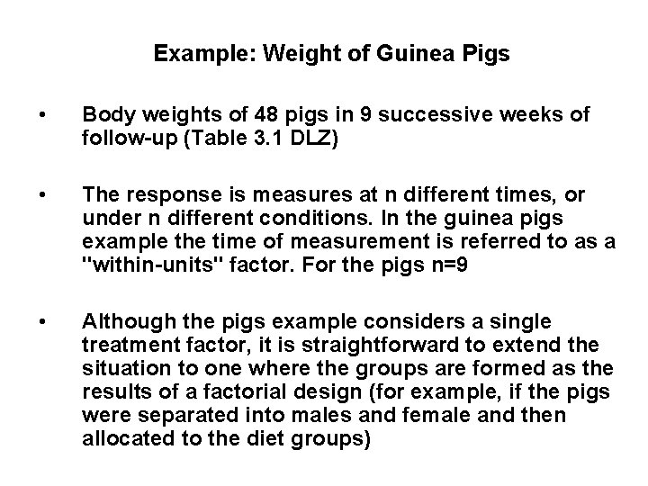
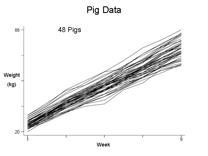
Example: Weight of Guinea Pigs • Body weights of 48 pigs in 9 successive weeks of follow-up (Table 3. 1 DLZ) • The response is measures at n different times, or under n different conditions. In the guinea pigs example the time of measurement is referred to as a "within-units" factor. For the pigs n=9 • Although the pigs example considers a single treatment factor, it is straightforward to extend the situation to one where the groups are formed as the results of a factorial design (for example, if the pigs were separated into males and female and then allocated to the diet groups)

Pig Data 48 Pigs Weight (kg) Week

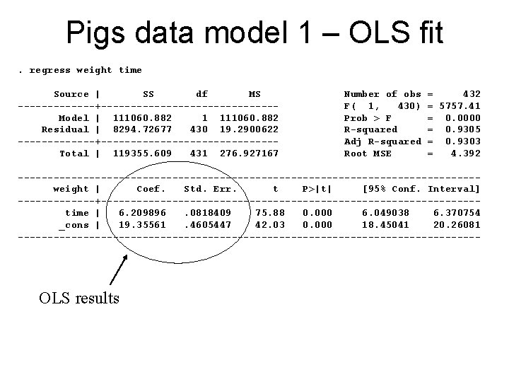
Pigs data model 1 – OLS fit. regress weight time Source | SS df MS -------+---------------Model | 111060. 882 1 111060. 882 Residual | 8294. 72677 430 19. 2900622 -------+---------------Total | 119355. 609 431 276. 927167 Number of obs F( 1, 430) Prob > F R-squared Adj R-squared Root MSE = 432 = 5757. 41 = 0. 0000 = 0. 9305 = 0. 9303 = 4. 392 ---------------------------------------weight | Coef. Std. Err. t P>|t| [95% Conf. Interval] -------+--------------------------------time | 6. 209896. 0818409 75. 88 0. 000 6. 049038 6. 370754 _cons | 19. 35561. 4605447 42. 03 0. 000 18. 45041 20. 26081 --------------------------------------- OLS results

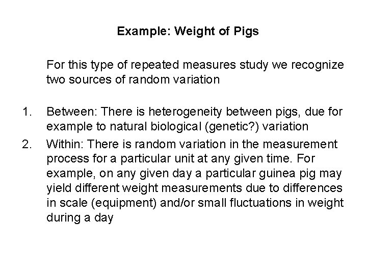
Example: Weight of Pigs For this type of repeated measures study we recognize two sources of random variation 1. 2. Between: There is heterogeneity between pigs, due for example to natural biological (genetic? ) variation Within: There is random variation in the measurement process for a particular unit at any given time. For example, on any given day a particular guinea pig may yield different weight measurements due to differences in scale (equipment) and/or small fluctuations in weight during a day

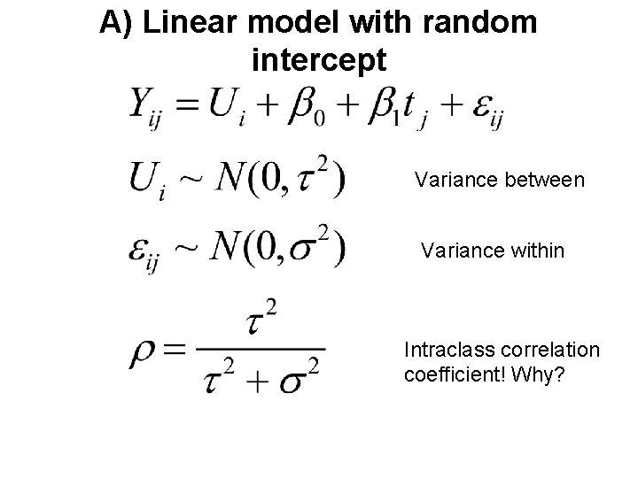
A) Linear model with random intercept Variance between Variance within Intraclass correlation coefficient! Why?

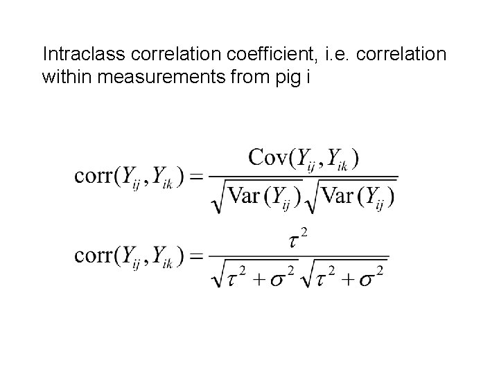
Intraclass correlation coefficient, i. e. correlation within measurements from pig i

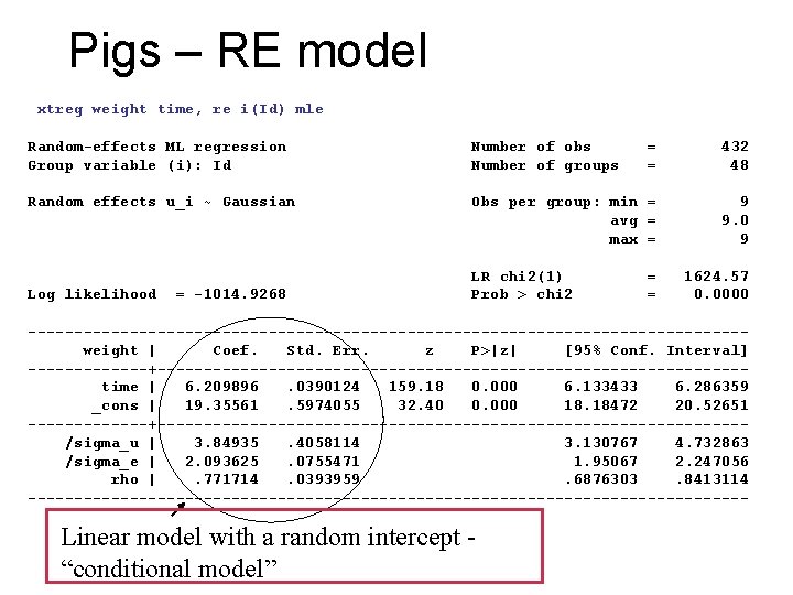
Pigs – RE model xtreg weight time, re i(Id) mle Random-effects ML regression Group variable (i): Id Number of obs Number of groups = = 432 48 Random effects u_i ~ Gaussian Obs per group: min = avg = max = 9 9. 0 9 Log likelihood = -1014. 9268 LR chi 2(1) Prob > chi 2 = = 1624. 57 0. 0000 ---------------------------------------weight | Coef. Std. Err. z P>|z| [95% Conf. Interval] -------+--------------------------------time | 6. 209896. 0390124 159. 18 0. 000 6. 133433 6. 286359 _cons | 19. 35561. 5974055 32. 40 0. 000 18. 18472 20. 52651 -------+--------------------------------/sigma_u | 3. 84935. 4058114 3. 130767 4. 732863 /sigma_e | 2. 093625. 0755471 1. 95067 2. 247056 rho |. 771714. 0393959. 6876303. 8413114 --------------------------------------- Linear model with a random intercept “conditional model”

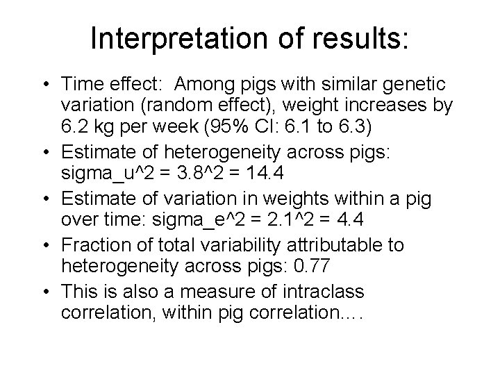
Interpretation of results: • Time effect: Among pigs with similar genetic variation (random effect), weight increases by 6. 2 kg per week (95% CI: 6. 1 to 6. 3) • Estimate of heterogeneity across pigs: sigma_u^2 = 3. 8^2 = 14. 4 • Estimate of variation in weights within a pig over time: sigma_e^2 = 2. 1^2 = 4. 4 • Fraction of total variability attributable to heterogeneity across pigs: 0. 77 • This is also a measure of intraclass correlation, within pig correlation….

Random Effects Model E[ Yi | Ui] = β 0+ β 1 time + Ui E[ Yi ] = β 0+ β 1 time

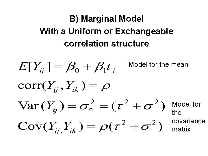
B) Marginal Model With a Uniform or Exchangeable correlation structure Model for the mean Model for the covariance matrix

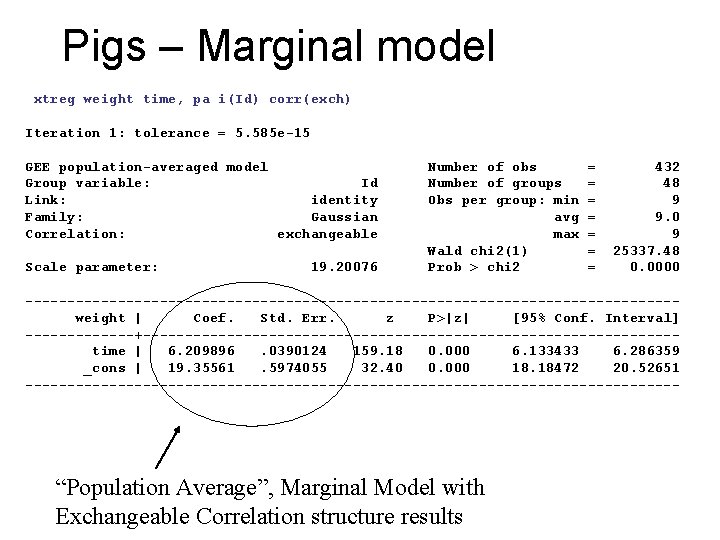
Pigs – Marginal model xtreg weight time, pa i(Id) corr(exch) Iteration 1: tolerance = 5. 585 e-15 GEE population-averaged model Group variable: Id Link: identity Family: Gaussian Correlation: exchangeable Scale parameter: 19. 20076 Number of obs Number of groups Obs per group: min avg max Wald chi 2(1) Prob > chi 2 = = = = 432 48 9 9. 0 9 25337. 48 0. 0000 ---------------------------------------weight | Coef. Std. Err. z P>|z| [95% Conf. Interval] -------+--------------------------------time | 6. 209896. 0390124 159. 18 0. 000 6. 133433 6. 286359 _cons | 19. 35561. 5974055 32. 40 0. 000 18. 18472 20. 52651 --------------------------------------- “Population Average”, Marginal Model with Exchangeable Correlation structure results

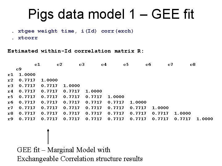
Pigs data model 1 – GEE fit. xtgee weight time, i(Id) corr(exch). xtcorr Estimated within-Id correlation matrix R: c 1 r 2 r 3 r 4 r 5 r 6 r 7 r 8 r 9 c 9 1. 0000 0. 7717 0. 7717 c 2 1. 0000 0. 7717 0. 7717 c 3 1. 0000 0. 7717 c 4 1. 0000 0. 7717 c 5 1. 0000 0. 7717 c 6 1. 0000 0. 7717 GEE fit – Marginal Model with Exchangeable Correlation structure results c 7 1. 0000 0. 7717 c 8 1. 0000 0. 7717 1. 0000

Marginal Model E[ Yi ] = β 0+ β 1 time

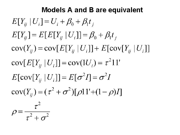
Models A and B are equivalent

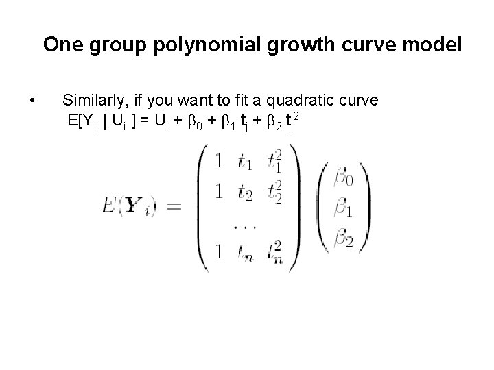
One group polynomial growth curve model • Similarly, if you want to fit a quadratic curve E[Yij | Ui ] = Ui + b 0 + b 1 tj + b 2 tj 2

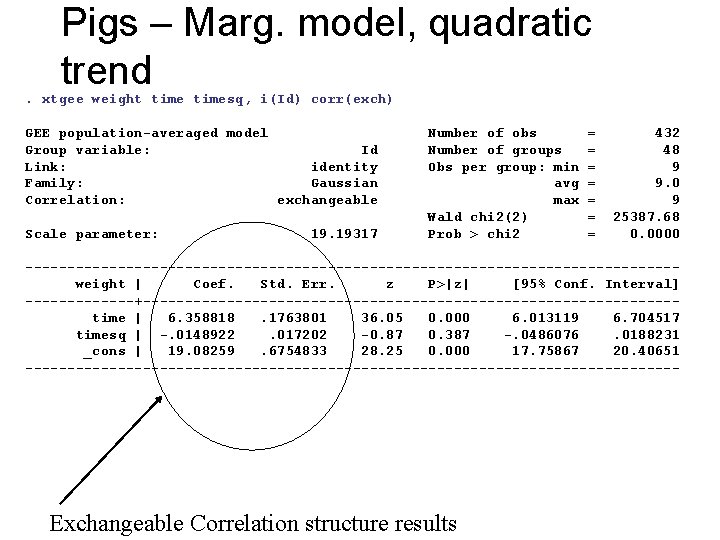
Pigs – Marg. model, quadratic trend . xtgee weight timesq, i(Id) corr(exch) GEE population-averaged model Group variable: Id Link: identity Family: Gaussian Correlation: exchangeable Scale parameter: 19. 19317 Number of obs Number of groups Obs per group: min avg max Wald chi 2(2) Prob > chi 2 = = = = 432 48 9 9. 0 9 25387. 68 0. 0000 ---------------------------------------weight | Coef. Std. Err. z P>|z| [95% Conf. Interval] -------+--------------------------------time | 6. 358818. 1763801 36. 05 0. 000 6. 013119 6. 704517 timesq | -. 0148922. 017202 -0. 87 0. 387 -. 0486076. 0188231 _cons | 19. 08259. 6754833 28. 25 0. 000 17. 75867 20. 40651 --------------------------------------- Exchangeable Correlation structure results

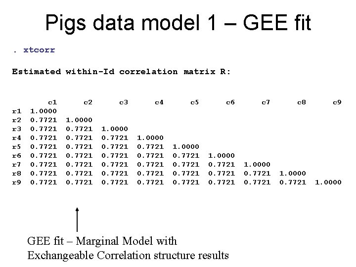
Pigs data model 1 – GEE fit. xtcorr Estimated within-Id correlation matrix R: r 1 r 2 r 3 r 4 r 5 r 6 r 7 r 8 r 9 c 1 1. 0000 0. 7721 0. 7721 c 2 c 3 c 4 c 5 c 6 c 7 c 8 c 9 1. 0000 0. 7721 0. 7721 1. 0000 0. 7721 1. 0000 GEE fit – Marginal Model with Exchangeable Correlation structure results

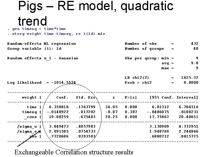
Pigs – RE model, quadratic trend . gen timesq = time*time. xtreg weight timesq, re i(Id) mle Random-effects ML regression Group variable (i): Id Number of obs Number of groups = = 432 48 Random effects u_i ~ Gaussian Obs per group: min = avg = max = 9 9. 0 9 Log likelihood = -1014. 5524 LR chi 2(2) Prob > chi 2 = = 1625. 32 0. 0000 ---------------------------------------weight | Coef. Std. Err. z P>|z| [95% Conf. Interval] -------+--------------------------------time | 6. 358818. 1763799 36. 05 0. 000 6. 01312 6. 704516 timesq | -. 0148922. 017202 -0. 87 0. 387 -. 0486075. 0188231 _cons | 19. 08259. 675483 28. 25 0. 000 17. 75867 20. 40651 -------+--------------------------------/sigma_u | 3. 849473. 4057983 3. 130909 4. 732951 /sigma_e | 2. 091585. 0754733 1. 948769 2. 244866 rho |. 7720686. 0393503. 6880712. 8415775 --------------------------------------- Exchangeable Correlation structure results

Random Effects Model E[ Yi | Ui] = β 0+ β 1 time + β 2 time 2 + Ui E[ Yi ] = ?

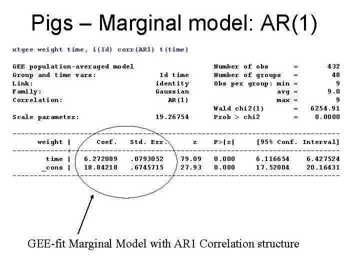
Pigs – Marginal model: AR(1) xtgee weight time, i(Id) corr(AR 1) t(time) GEE population-averaged model Group and time vars: Link: Family: Correlation: Id time identity Gaussian AR(1) Scale parameter: 19. 26754 Number of obs Number of groups Obs per group: min avg max Wald chi 2(1) Prob > chi 2 = = = = 432 48 9 9. 0 9 6254. 91 0. 0000 ---------------------------------------weight | Coef. Std. Err. z P>|z| [95% Conf. Interval] -------+--------------------------------time | 6. 272089. 0793052 79. 09 0. 000 6. 116654 6. 427524 _cons | 18. 84218. 6745715 27. 93 0. 000 17. 52004 20. 16431 --------------------------------------- GEE-fit Marginal Model with AR 1 Correlation structure

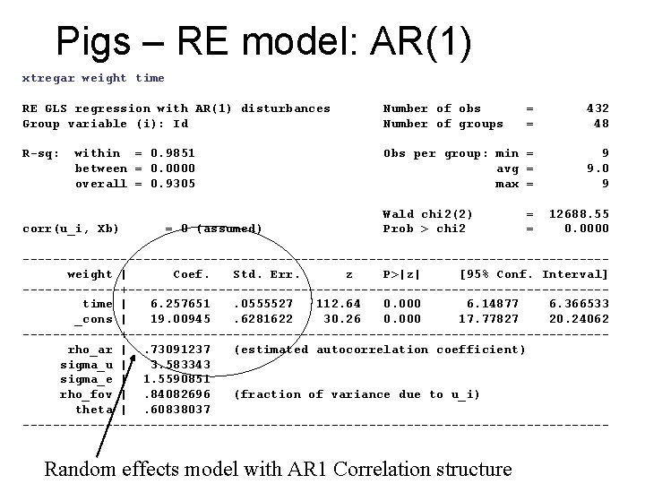
Pigs – RE model: AR(1) xtregar weight time RE GLS regression with AR(1) disturbances Group variable (i): Id Number of obs Number of groups = = 432 48 R-sq: Obs per group: min = avg = max = 9 9. 0 9 within = 0. 9851 between = 0. 0000 overall = 0. 9305 corr(u_i, Xb) = 0 (assumed) Wald chi 2(2) Prob > chi 2 = = 12688. 55 0. 0000 ---------------------------------------weight | Coef. Std. Err. z P>|z| [95% Conf. Interval] -------+--------------------------------time | 6. 257651. 0555527 112. 64 0. 000 6. 14877 6. 366533 _cons | 19. 00945. 6281622 30. 26 0. 000 17. 77827 20. 24062 -------+--------------------------------rho_ar |. 73091237 (estimated autocorrelation coefficient) sigma_u | 3. 583343 sigma_e | 1. 5590851 rho_fov |. 84082696 (fraction of variance due to u_i) theta |. 60838037 --------------------------------------- Random effects model with AR 1 Correlation structure

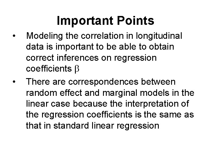
Important Points • • Modeling the correlation in longitudinal data is important to be able to obtain correct inferences on regression coefficients b There are correspondences between random effect and marginal models in the linear case because the interpretation of the regression coefficients is the same as that in standard linear regression

Example using Stata:

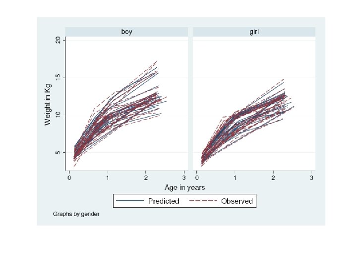
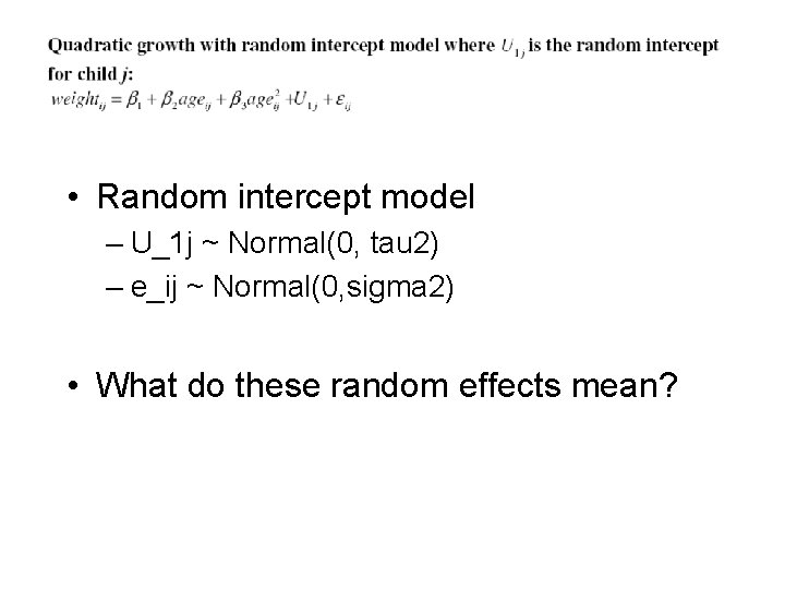
• Random intercept model – U_1 j ~ Normal(0, tau 2) – e_ij ~ Normal(0, sigma 2) • What do these random effects mean?

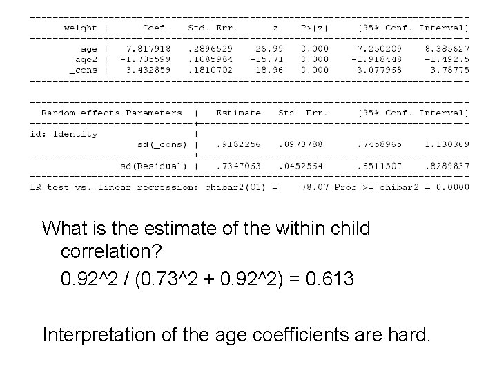
What is the estimate of the within child correlation? 0. 92^2 / (0. 73^2 + 0. 92^2) = 0. 613 Interpretation of the age coefficients are hard.

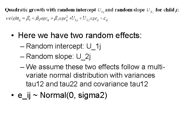
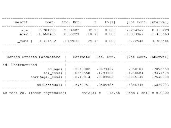
• Here we have two random effects: – Random intercept: U_1 j – Random slope: U_2 j – We assume these two effects follow a multivariate normal distribution with variances tau 12 and tau 22 and covariance tau 12 • e_ij ~ Normal(0, sigma 2)

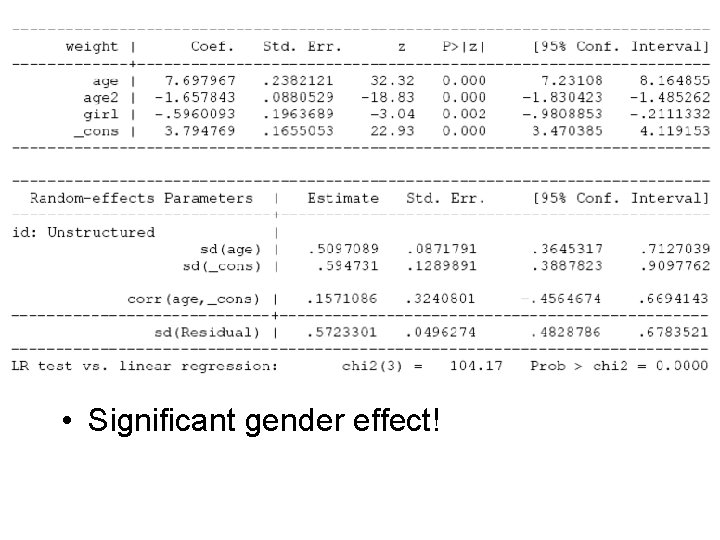
• Significant gender effect!