LECTURE 2 Keynesian Income Determination 1 Aggregate Expenditure

LECTURE 2 Keynesian Income Determination 1

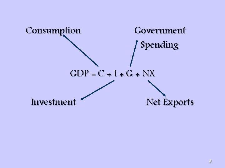
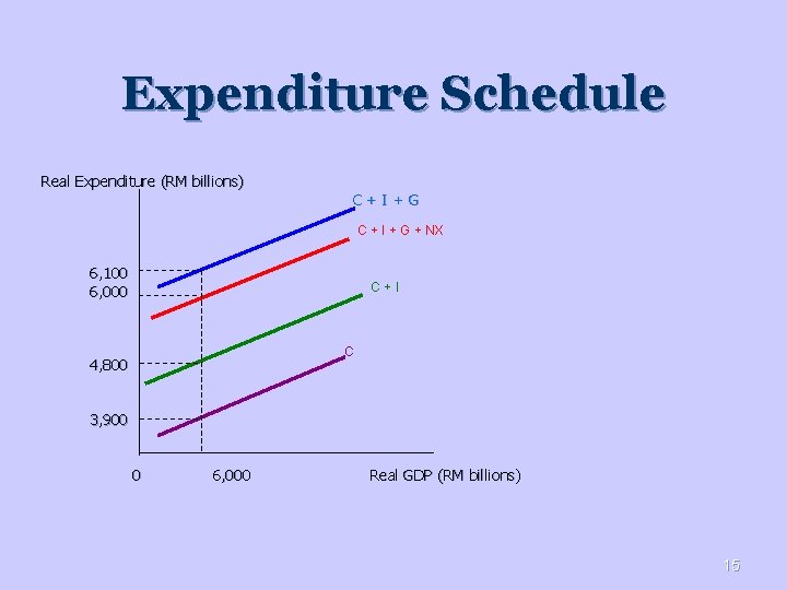
Aggregate Expenditure n n Defined as the total amount that firms and households plan to spend on goods and services at each level of income. It can also be seen that the aggregate expenditure is the sum of expenditures on consumption, investment, government expenses and net exports. 2

Consumption Government Spending GDP = C + I + G + NX Investment Net Exports 3

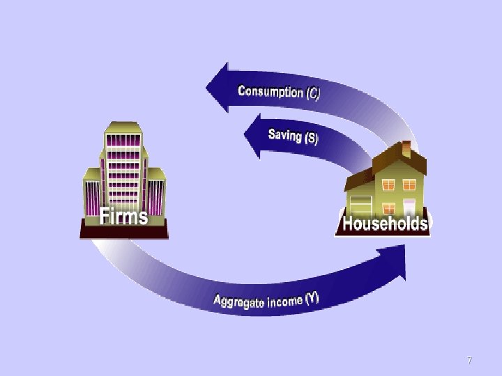
Income, Savings and their Determinants A household can do 2 things with income: (a) consume – buy goods and services. (b) save. n Saving is the part of its income that a household does not consume in a given period. n 4

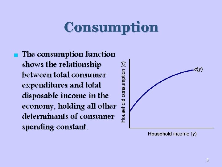
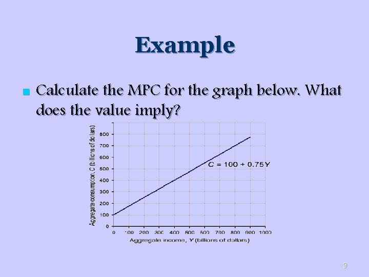
Consumption n The consumption function shows the relationship between total consumer expenditures and total disposable income in the economy, holding all other determinants of consumer spending constant. 5

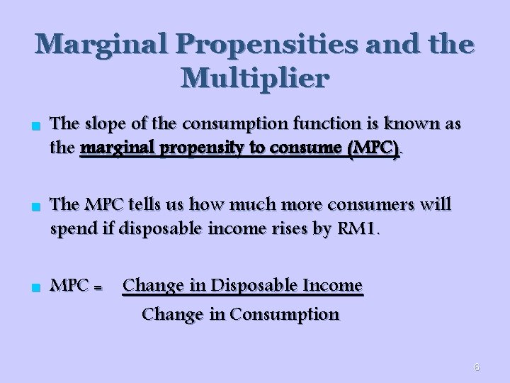
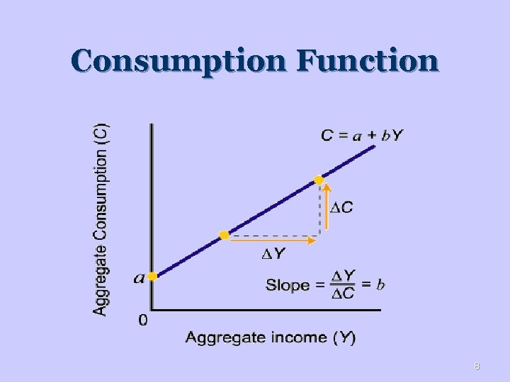
Marginal Propensities and the Multiplier n n n The slope of the consumption function is known as the marginal propensity to consume (MPC). The MPC tells us how much more consumers will spend if disposable income rises by RM 1. MPC = Change in Disposable Income Change in Consumption 6

7

Consumption Function 8

Example n Calculate the MPC for the graph below. What does the value imply? 9

Factors that Shift the Consumption Function n n Any change in disposable income will cause a movement along the same consumption function, where else a change in other determinants will shift the consumption function. Wealth Price level Real interest rate Future income expectation 10

Wealth n n A source of purchasing power in addition to income. Eg. A wealthy retiree with a huge bank balance may earn little current income when interest rates are low. But a high-flying investment banker who spends every penny of high income she earns will not accumulate much wealth. 11

Price Level n n n People hold a great deal of wealth in forms that are fixed in money terms. Bank accounts are the most obvious example, but government and corporate bonds also have fixed values in money terms. The purchasing power of such money-fixed assets obviously declines whenever the price level rises, which means that the asset can buy less. Eg. If the price level rises by 10%, a RM 1, 000 government bond will buy 10% less than it could when prices were lower. 12

n n Real Interest Rate A higher real rate of interest raises the rewards for saving and vice versa. Future Income Expectation When consumers expect income to increase in the future, current consumption will also increase and vice versa. 13

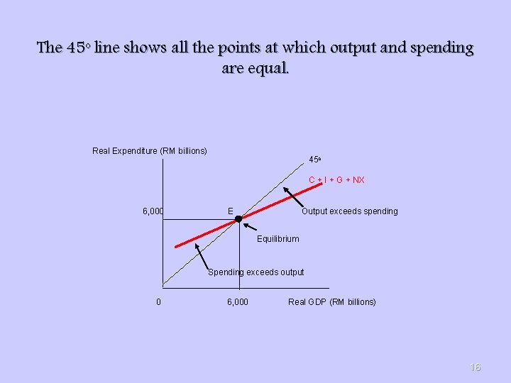
Equilibrium GDP Determination n Equilibrium GDP is that output level at which the total amount of goods and services produced, GDP, is just equal to the total amount of goods purchased. 14

Expenditure Schedule Real Expenditure (RM billions) C+I+G C + I + G + NX 6, 100 6, 000 C+I C 4, 800 3, 900 0 6, 000 Real GDP (RM billions) 15

The 45 o line shows all the points at which output and spending are equal. Real Expenditure (RM billions) 45 o C + I + G + NX 6, 000 E Output exceeds spending Equilibrium Spending exceeds output 0 6, 000 Real GDP (RM billions) 16

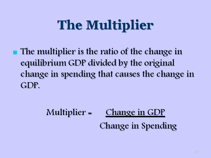
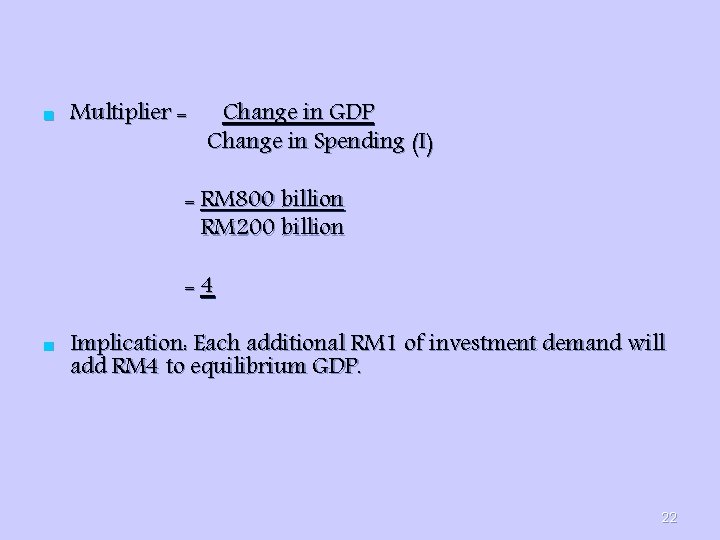
The Multiplier n The multiplier is the ratio of the change in equilibrium GDP divided by the original change in spending that causes the change in GDP. Multiplier = Change in GDP Change in Spending 17

n The remarkable thing about the multiplier is that it shows that a change in spending will bring about an even larger change in equilibrium GDP on the demand side. 18

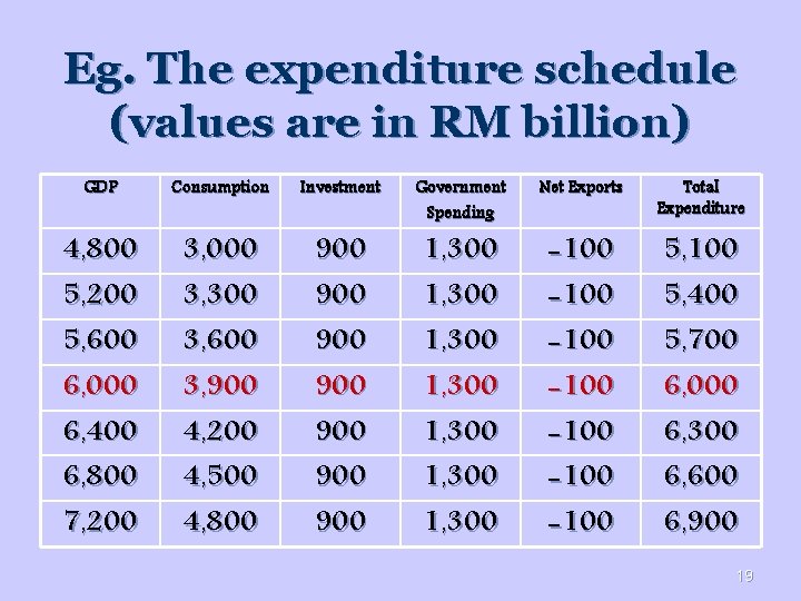
Eg. The expenditure schedule (values are in RM billion) GDP Consumption Investment 4, 800 5, 200 5, 600 6, 000 6, 400 6, 800 7, 200 3, 000 3, 300 3, 600 3, 900 4, 200 4, 500 4, 800 900 900 Government Spending 1, 300 1, 300 Net Exports Total Expenditure -100 -100 5, 400 5, 700 6, 000 6, 300 6, 600 6, 900 19

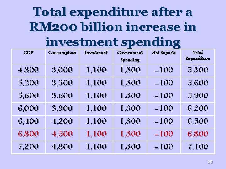
Total expenditure after a RM 200 billion increase in investment spending GDP Consumption Investment 4, 800 5, 200 5, 600 6, 000 6, 400 6, 800 7, 200 3, 000 3, 300 3, 600 3, 900 4, 200 4, 500 4, 800 1, 100 1, 100 Government Spending 1, 300 1, 300 Net Exports Total Expenditure -100 -100 5, 300 5, 600 5, 900 6, 200 6, 500 6, 800 7, 100 20

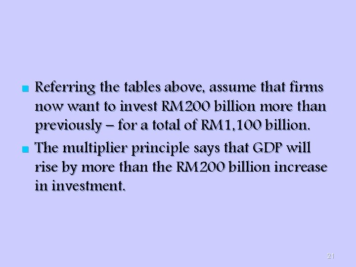
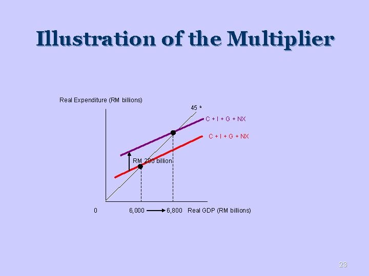
n n Referring the tables above, assume that firms now want to invest RM 200 billion more than previously – for a total of RM 1, 100 billion. The multiplier principle says that GDP will rise by more than the RM 200 billion increase in investment. 21

n Multiplier = Change in GDP Change in Spending (I) = RM 800 billion RM 200 billion =4 n Implication: Each additional RM 1 of investment demand will add RM 4 to equilibrium GDP. 22

Illustration of the Multiplier Real Expenditure (RM billions) 45 o C + I + G + NX RM 200 billion 0 6, 000 6, 800 Real GDP (RM billions) 23