Macroeconomics Module 10 The IncomeExpenditure Model The IncomeExpenditure

Macroeconomics Module 10: The Income-Expenditure Model

The Income-Expenditure Model • • • The Keynesian view of macroeconomics was developed during the Great Depression in the 1930 s, long before the AD–AS model was popularized. Keynesian economics was traditionally explained with a different approach, known as the Income-Expenditure, or Keynesian Cross model. The Keynesian-Cross model is still useful today because it provides a much more detailed and intuitive explanation of aggregate demand than is given in the AD-AS model. • • • It provides a richer understanding of the components of aggregate expenditure: consumption, investment, government spending, and net exports It teaches more about what causes recessionary and inflationary gaps It explains the expenditure multiplier

The Key Role of Aggregate Expenditure • • Aggregate Expenditure Function: graphical relationship between national income as a function of aggregate expenditure, which is defined as consumption plus investment plus government spending plus net exports Aggregate Expenditure Schedule: aggregate expenditure function expressed as a table

The Income-Expenditure Model (cont. ) • • • The fundamental assumption of Keynesian economics is that economic activity, that is, output and employment, are determined primarily by the amount of aggregate demand (or total spending) in the economy The model makes no explicit mention of aggregate supply or of the price level Remember that GDP can be thought of in several equivalent ways: • • Measures both the value of spending on final goods The value of the production of final goods

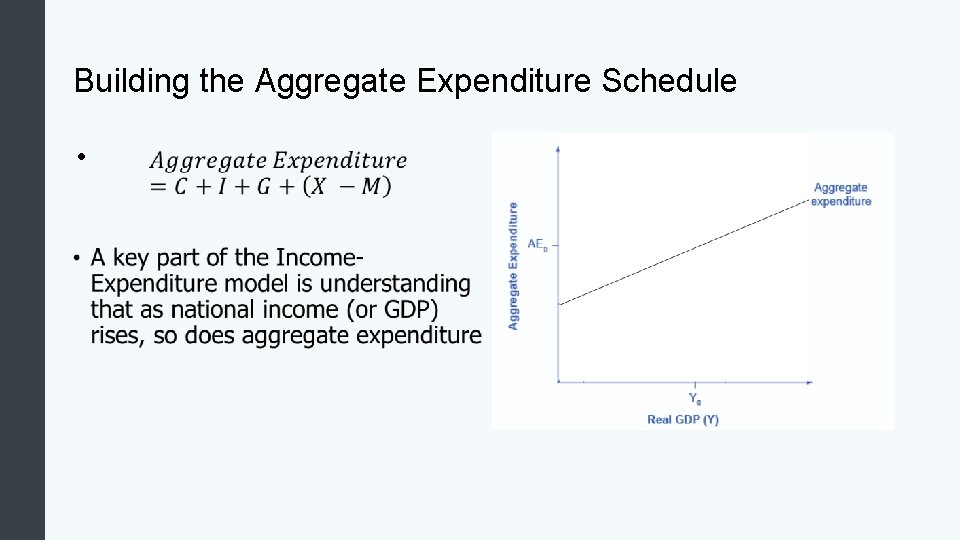
Building the Aggregate Expenditure Schedule •

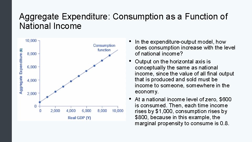
Aggregate Expenditure: Consumption • • Autonomous Consumption: The amount consumers spend if their income was zero; i. e. consumer spending which is caused by something other than income, for example, borrowing Consumption Function: graphical relationship between national income and consumption expenditure; algebraically: C = a + MPC*Y, where a is autonomous consumption (the amount of consumption expenditure when Y = 0), MPC is the marginal propensity to consume, and Y is national income Marginal Propensity to Consume: fraction of any change in income which is spent; algebraically MPC = ΔC/ΔY Marginal Propensity to Save: fraction of any change in income which is saved; algebraically MPS = ΔS/ΔY

Aggregate Expenditure: Consumption as a Function of National Income • • • In the expenditure-output model, how does consumption increase with the level of national income? Output on the horizontal axis is conceptually the same as national income, since the value of all final output that is produced and sold must be income to someone, somewhere in the economy. At a national income level of zero, $600 is consumed. Then, each time income rises by $1, 000, consumption rises by $800, because in this example, the marginal propensity to consume is 0. 8.

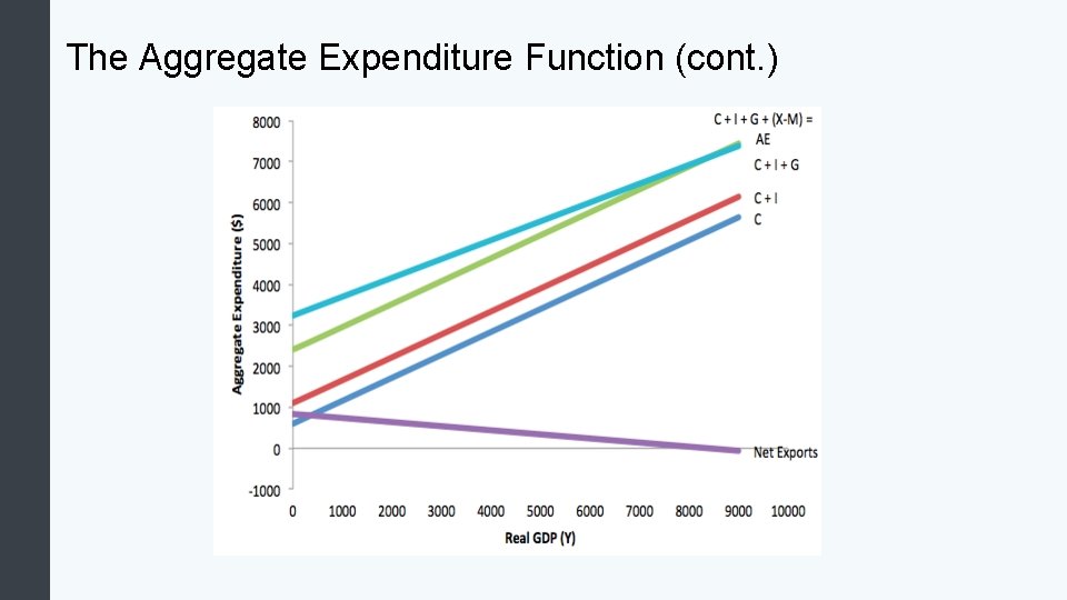
Aggregate Expenditure: Investment, Government Spending, and Net Exports • • Aggregate Expenditure Function: graphical relationship between national income as a function of aggregate expenditure, which is defined as consumption plus investment plus government spending plus net exports Aggregate Expenditure Schedule: aggregate expenditure function expressed as a table Autonomous Expenditures: all the components of aggregate expenditure, which do not vary with national income; these include autonomous consumption, investment, government, and export expenditures Government Spending Function: horizontal line showing the relationship between national income and government spending Investment Expenditure Function: horizontal line showing the relationship between national income and government spending Marginal Propensity to Import: fraction of any change in income which is spent; algebraically MPI =ΔM /ΔY Net Export Function: graphical relationship between national income and net exports (export expenditures minus import expenditures)

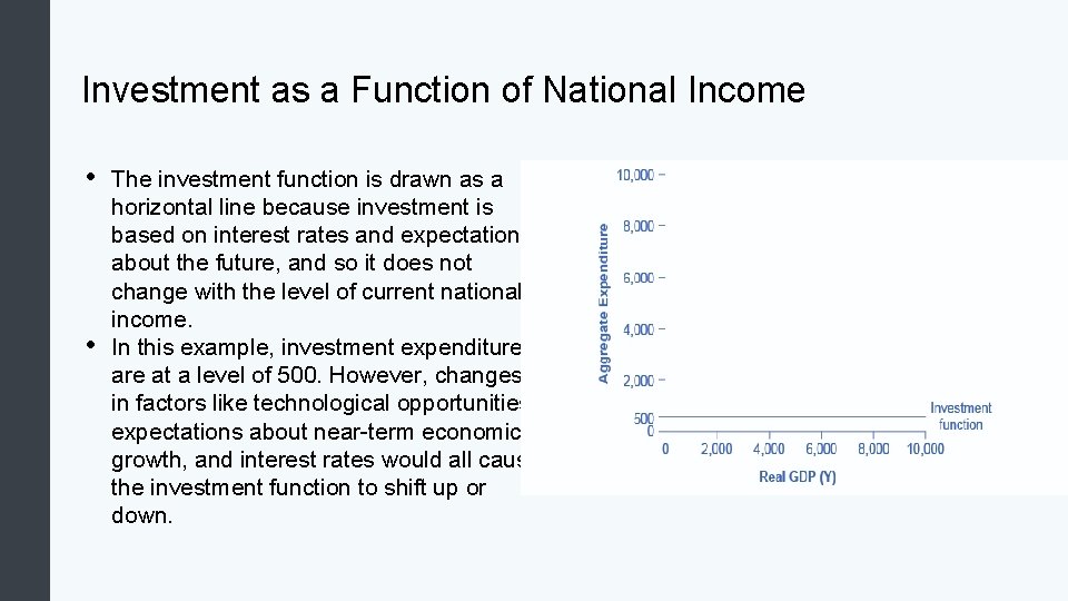
Investment as a Function of National Income • • The investment function is drawn as a horizontal line because investment is based on interest rates and expectations about the future, and so it does not change with the level of current national income. In this example, investment expenditures are at a level of 500. However, changes in factors like technological opportunities, expectations about near-term economic growth, and interest rates would all cause the investment function to shift up or down.

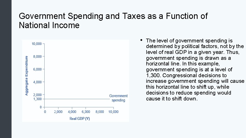
Government Spending and Taxes as a Function of National Income • The level of government spending is determined by political factors, not by the level of real GDP in a given year. Thus, government spending is drawn as a horizontal line. In this example, government spending is at a level of 1, 300. Congressional decisions to increase government spending will cause this horizontal line to shift up, while decisions to reduce spending would cause it to shift down.

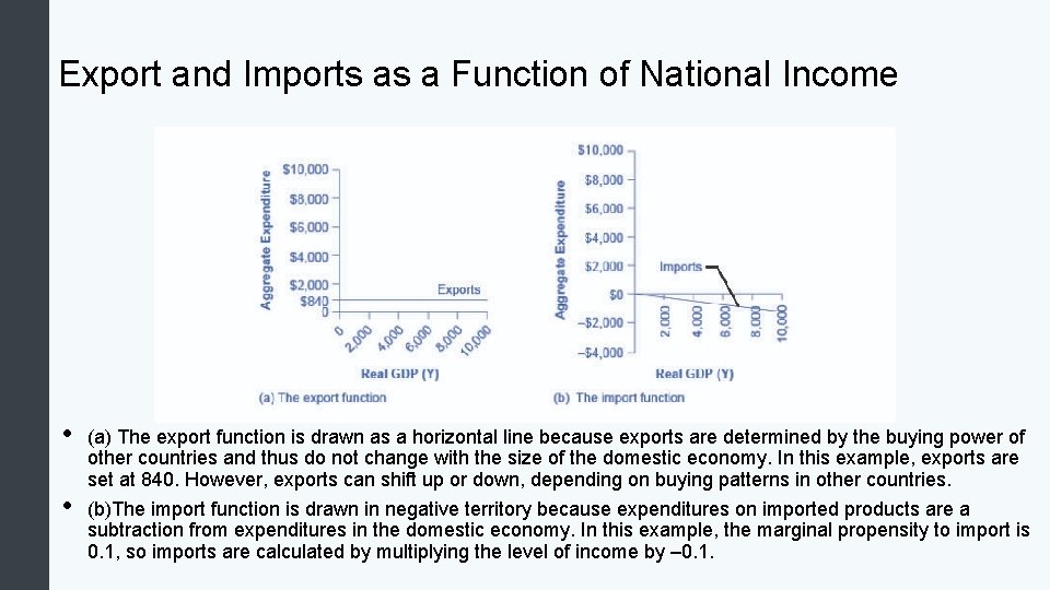
Export and Imports as a Function of National Income • • (a) The export function is drawn as a horizontal line because exports are determined by the buying power of other countries and thus do not change with the size of the domestic economy. In this example, exports are set at 840. However, exports can shift up or down, depending on buying patterns in other countries. (b)The import function is drawn in negative territory because expenditures on imported products are a subtraction from expenditures in the domestic economy. In this example, the marginal propensity to import is 0. 1, so imports are calculated by multiplying the level of income by – 0. 1.

The Aggregate Expenditure Function

The Aggregate Expenditure Function (cont. )

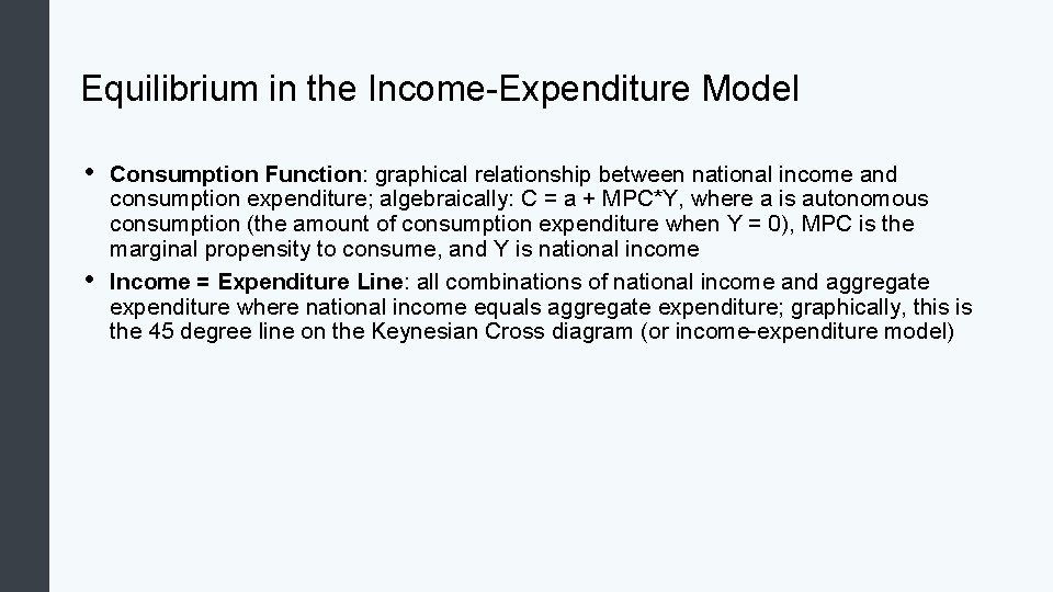
Equilibrium in the Income-Expenditure Model • • Consumption Function: graphical relationship between national income and consumption expenditure; algebraically: C = a + MPC*Y, where a is autonomous consumption (the amount of consumption expenditure when Y = 0), MPC is the marginal propensity to consume, and Y is national income Income = Expenditure Line: all combinations of national income and aggregate expenditure where national income equals aggregate expenditure; graphically, this is the 45 degree line on the Keynesian Cross diagram (or income-expenditure model)

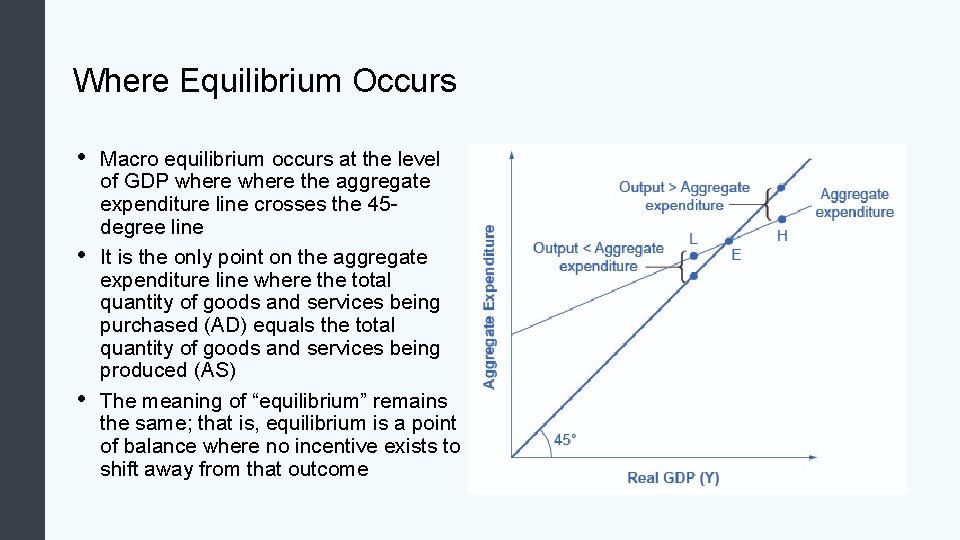
Where Equilibrium Occurs • • • Macro equilibrium occurs at the level of GDP where the aggregate expenditure line crosses the 45 degree line It is the only point on the aggregate expenditure line where the total quantity of goods and services being purchased (AD) equals the total quantity of goods and services being produced (AS) The meaning of “equilibrium” remains the same; that is, equilibrium is a point of balance where no incentive exists to shift away from that outcome

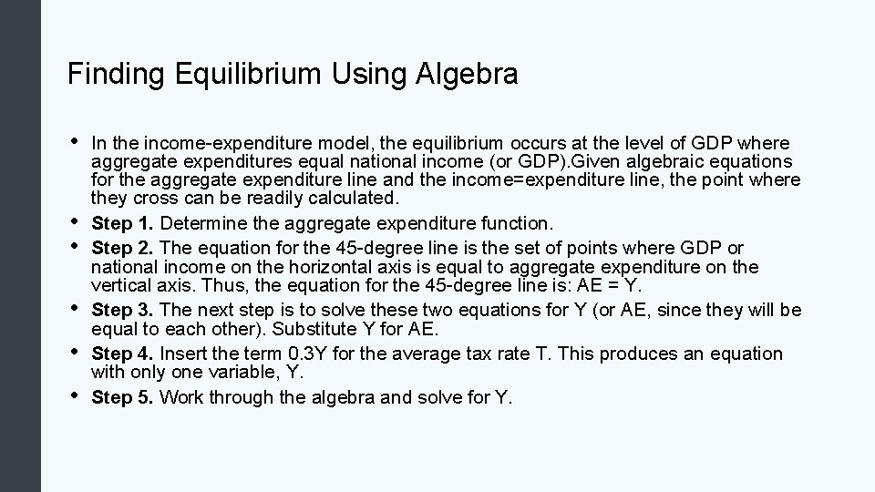
Finding Equilibrium Using Algebra • • • In the income-expenditure model, the equilibrium occurs at the level of GDP where aggregate expenditures equal national income (or GDP). Given algebraic equations for the aggregate expenditure line and the income=expenditure line, the point where they cross can be readily calculated. Step 1. Determine the aggregate expenditure function. Step 2. The equation for the 45 -degree line is the set of points where GDP or national income on the horizontal axis is equal to aggregate expenditure on the vertical axis. Thus, the equation for the 45 -degree line is: AE = Y. Step 3. The next step is to solve these two equations for Y (or AE, since they will be equal to each other). Substitute Y for AE. Step 4. Insert the term 0. 3 Y for the average tax rate T. This produces an equation with only one variable, Y. Step 5. Work through the algebra and solve for Y.

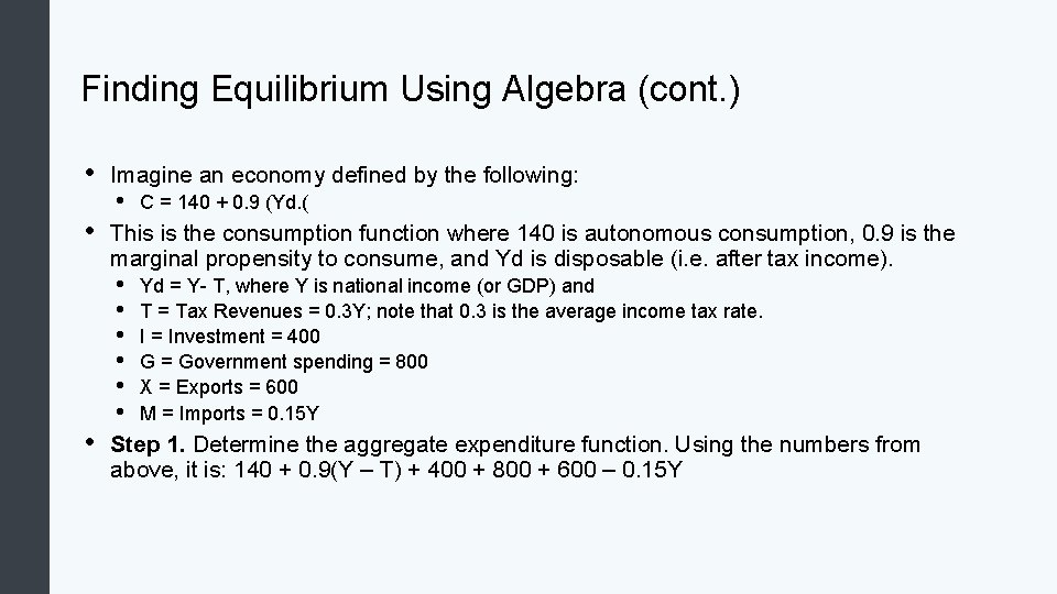
Finding Equilibrium Using Algebra (cont. ) • • • Imagine an economy defined by the following: • C = 140 + 0. 9 (Yd. ( This is the consumption function where 140 is autonomous consumption, 0. 9 is the marginal propensity to consume, and Yd is disposable (i. e. after tax income). • • • Yd = Y- T, where Y is national income (or GDP) and T = Tax Revenues = 0. 3 Y; note that 0. 3 is the average income tax rate. I = Investment = 400 G = Government spending = 800 X = Exports = 600 M = Imports = 0. 15 Y Step 1. Determine the aggregate expenditure function. Using the numbers from above, it is: 140 + 0. 9(Y – T) + 400 + 800 + 600 – 0. 15 Y

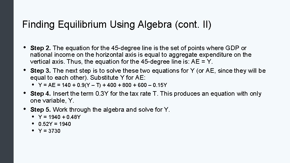
Finding Equilibrium Using Algebra (cont. II) • • Step 2. The equation for the 45 -degree line is the set of points where GDP or national income on the horizontal axis is equal to aggregate expenditure on the vertical axis. Thus, the equation for the 45 -degree line is: AE = Y. Step 3. The next step is to solve these two equations for Y (or AE, since they will be equal to each other). Substitute Y for AE: • Y = AE = 140 + 0. 9(Y – T) + 400 + 800 + 600 – 0. 15 Y Step 4. Insert the term 0. 3 Y for the tax rate T. This produces an equation with only one variable, Y. Step 5. Work through the algebra and solve for Y. • • • Y = 1940 + 0. 48 Y 0. 52 Y = 1940 Y = 3730

Recessionary and Inflationary Gaps in the Income. Expenditure Model • • • Inflationary Gap: when macro equilibrium occurs at a level of GDP greater than potential GDP; thus, unemployment is lower than the natural rate Potential GDP Line: vertical line on the Keynesian Cross diagram indicating where GDP (on the horizontal axis) is at potential Recessionary Gap: when macro equilibrium occurs at a level of GDP less than potential GDP; thus, unemployment is higher than the natural rate

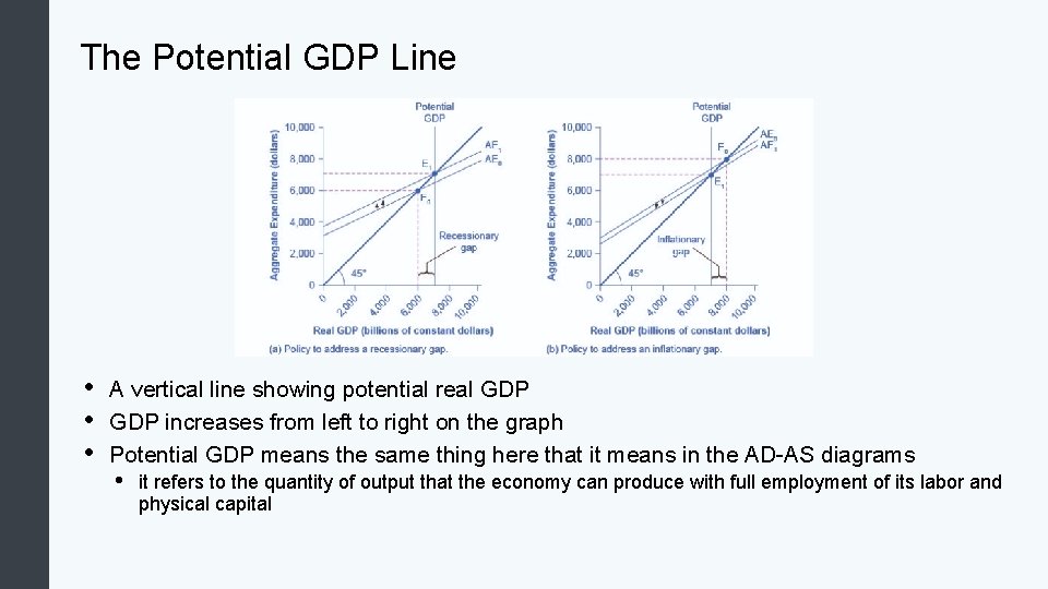
The Potential GDP Line • • • A vertical line showing potential real GDP increases from left to right on the graph Potential GDP means the same thing here that it means in the AD-AS diagrams • it refers to the quantity of output that the economy can produce with full employment of its labor and physical capital

Recessionary and Inflationary Gaps • • • In the Keynesian cross diagram, if the aggregate expenditure line intersects the 45 degree line at the level of potential GDP, then the economy is in sound shape The equilibrium might be higher or lower. What might cause a recessionary gap? • Anything that shifts the aggregate expenditure line down is a potential cause of recession, including a decline in consumption, a rise in savings, a fall in investment, a drop in government spending or a rise in taxes, or a fall in exports or a rise in imports

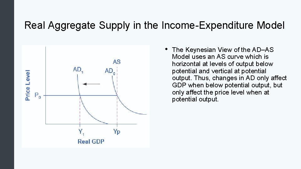
Real Aggregate Supply in the Income-Expenditure Model • The Keynesian View of the AD–AS Model uses an AS curve which is horizontal at levels of output below potential and vertical at potential output. Thus, changes in AD only affect GDP when below potential output, but only affect the price level when at potential output.

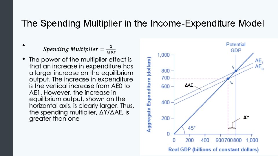
The Spending Multiplier in the Income-Expenditure Model •

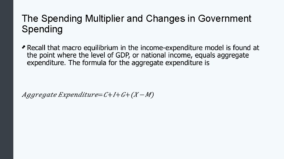
The Spending Multiplier and Changes in Government Spending •

Quick Review • • What are the components of aggregate expenditure and their importance in the income-expenditure model? Explain and graph the consumption function. What would cause the consumption function to grow steeper or flatter, or to shift up or down? What are the investment, government spending, and net export functions? How is the aggregate expenditure curve constructed from the consumption, investment, government spending and net export functions? Explain macro equilibrium using the income-expenditure model. Identify macro equilibrium graphically and using tables. How do you find the macro equilibrium using algebra?

More Quick Review • • • How do you define potential real GDP and be able to draw and explain the potential GDP line? Identify appropriate Keynesian policies in response to recessionary and inflationary gaps. Explain aggregate supply in the income-expenditure model and how the incomeexpenditure model correlates to the AD-AS model. Explain and demonstrate the multiplier graphically using the income-expenditure model. How do you determine how government spending should change to reach equilibrium, or full employment (using the income-expenditure model)?