LEASTSQUARES REGRESSION 3 2 Role of s and

- Slides: 10

LEAST-SQUARES REGRESSION 3. 2 Role of s and r 2 in Regression

REVIEW FROM LAST WEEK • Plot Scatterplot • Find Correlation and LSRL • Graph LSRL • Look at Residual Plot to determine if LSRL is a good fit

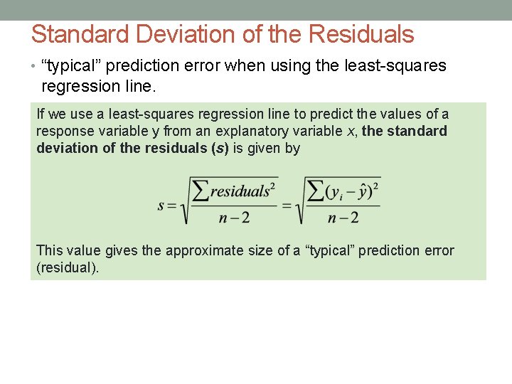
Standard Deviation of the Residuals • “typical” prediction error when using the least-squares regression line. If we use a least-squares regression line to predict the values of a response variable y from an explanatory variable x, the standard deviation of the residuals (s) is given by This value gives the approximate size of a “typical” prediction error (residual).

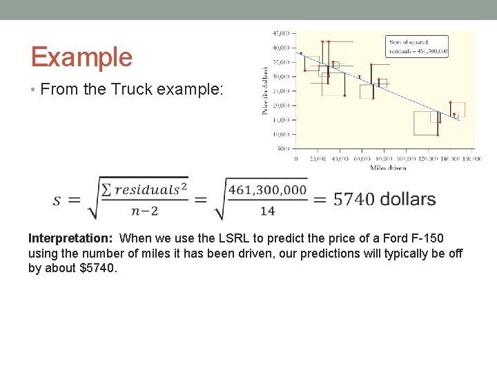
Example • From the Truck example: Interpretation: When we use the LSRL to predict the price of a Ford F-150 using the number of miles it has been driven, our predictions will typically be off by about $5740.

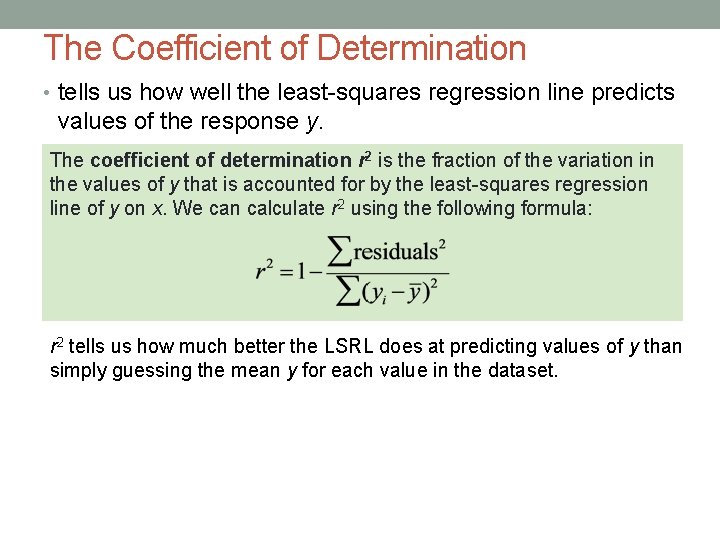
The Coefficient of Determination • tells us how well the least-squares regression line predicts values of the response y. The coefficient of determination r 2 is the fraction of the variation in the values of y that is accounted for by the least-squares regression line of y on x. We can calculate r 2 using the following formula: r 2 tells us how much better the LSRL does at predicting values of y than simply guessing the mean y for each value in the dataset.

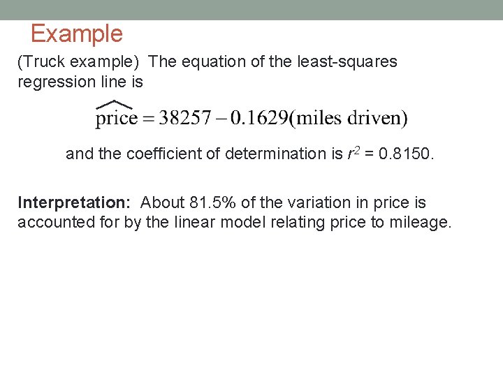
Example (Truck example) The equation of the least-squares regression line is and the coefficient of determination is r 2 = 0. 8150. Interpretation: About 81. 5% of the variation in price is accounted for by the linear model relating price to mileage.

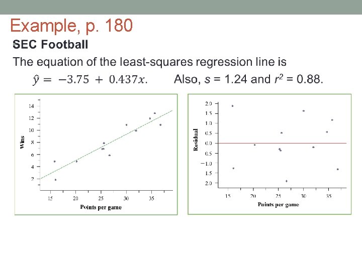
Example, p. 180 •

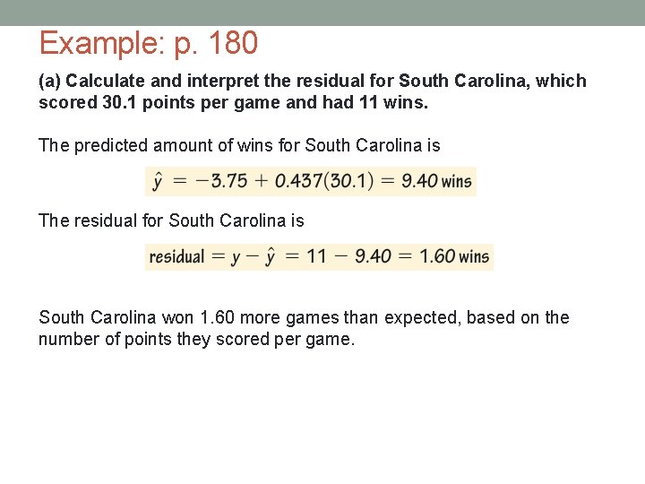
Example: p. 180 (a) Calculate and interpret the residual for South Carolina, which scored 30. 1 points per game and had 11 wins. The predicted amount of wins for South Carolina is The residual for South Carolina is South Carolina won 1. 60 more games than expected, based on the number of points they scored per game.

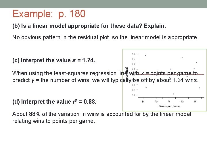
Example: p. 180 (b) Is a linear model appropriate for these data? Explain. No obvious pattern in the residual plot, so the linear model is appropriate. (c) Interpret the value s = 1. 24. When using the least-squares regression line with x = points per game to predict y = the number of wins, we will typically be off by about 1. 24 wins. (d) Interpret the value r 2 = 0. 88. About 88% of the variation in wins is accounted for by the linear model relating wins to points per game.

HW: Due on Friday • p. 195 # 55, 78