INVENTORY MODELS FOR INDEPENDENT DEMAND DEPENDENT AND INDEPENDENT

INVENTORY MODELS FOR INDEPENDENT DEMAND

DEPENDENT AND INDEPENDENT DEMAND • Independent demand is demand for a finished product, such as a computer, a bicycle, or a pizza. • Dependent demand, on the other hand, is demand for component parts or subassemblies. For example, this would be the microchips in the computer, the wheels on the bicycle, or the cheese on the pizza.

INVENTORY MODELS FOR INDEPENDENT DEMAND We are going to use the Basic Economic Order Quantity(EOQ) and the Production Order Quantity Model, to answer to the next questions: • When to order? • How much to order?

THE BASIC ECONOMIC ORDER QUANTITY (EOQ) It is one of the oldest and most commonly known inventory control techniques. it has several assumptions: • Demand is known • Lead time • Receipts are instantaneous and complete • No quantity discounts • Setup costs and holding costs are variable costs • Stockout can be avoided

OBJECTIVE OF INVENTORY MODELS -> MINIMIZE TOTAL COST

To obtain the Q* are necessary some steps 1. 2. 3. 4. Develop an expression for setup or ordering cost Develop an expression for holding cost Set setup cost equal to holding cost Solve the equation for the optimal order quantity

Variables: • • • Q = Number of units per order Q* = the optimal number of units per order (EOQ) D = Annual demand in units for the inventory item S = setup or ordering cost for each order H = holding or carrying costper unit per year

Expected number of order (N) = Demand/Order Quantity = D/Q* Expercted time between orders (T) = Number of working days per year/ N Total annual cost = Setup cost + Holding cost

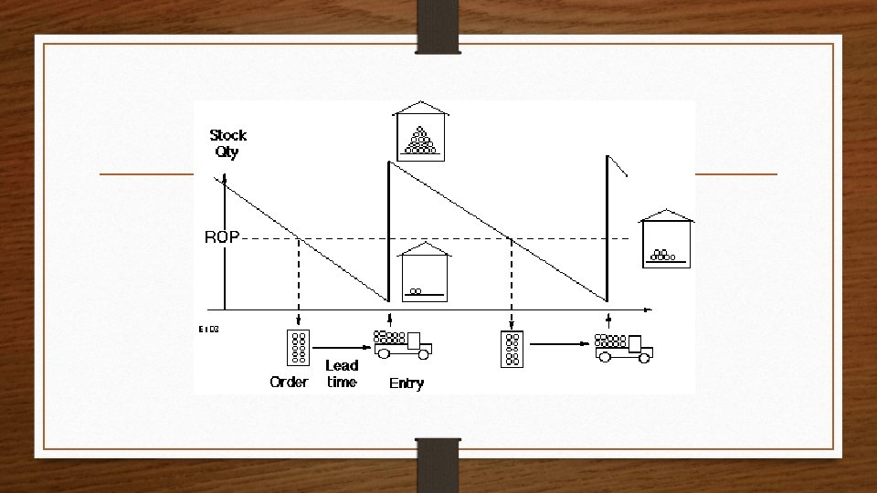
REORDER POINT • Simple inventory model assume that receipt of an order is instantaneous HOWEVER • The time between placement and receipt of an order, lead time (or delivery time), take time (shorter or longer) • The when-to-order decision is usually expressed in terms of a reorder point (ROP)

ROP Thus , the when-to-order decision is usually expressed in terms of a reorder point (ROP) --> the inventory level at which an order should be placed This equation for ROP assumes that demand during lead time and lead time itself are constant. When this is not the case we should add the safety stock. • ROP = (Demand per day) x (Lead time for a new order in days) = d x. L • The demand per day (d) = D/Number of working days in a year

EXERCISE • Sharp Inc; a company that markets hypodermic needles to hospitals would like to reduce its inventory cost by determining the optimal number of hypodermic needles to obtain per order. The annual demand is 1000 units, the setup cost or ordering cost is $10 per order, and the holding cost per unit per year is $0. 50. Assuming that the company has a 250 – day working year, calculate: • • • The optimal number of units per order The number of orders The expected time between orders Demand per day. The reorder point. Determine the combined annual ordering and holding cost

ROBUST MODEL A benefit of the EOQ model is that it is robust, that means that it gives satisfactory answer even with substantial variation in parameters, so variations in setup costs, holding costs, demand, or even EOQ make relatively modest differences in total cost.

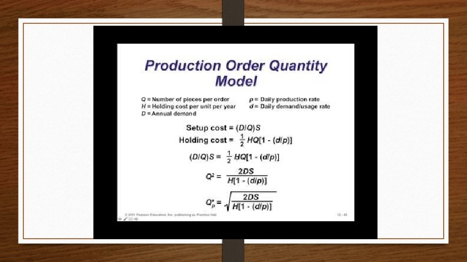
PRODUCTION ORDER QUANTITY MODEL This model is applicable when the inventory is received over a period a time, under two situatios: 1. When inventory continuosly flows or build up over a period of time after an order has been placed. 2. When units are produced and sold simultaneously.

1. (Annual inventory holding cost) = (Average inventory level) x H 2. (Average inventory level) = (Maximum inventory level)/2 3. (Maximum inventory level) = Q(1 - d/p) 4. Annual inventory holding cost = (Max. inventory level)/2 x (H)

EXERCISE Nathan Manufacturing, Inc. , makes and sells specialty hubcaps for the retail automobile aftermarket. A Nathan's forecast for its wirg wheel hubcap is 1, 000 units next year, with an average daily demand of 4 units. However, the production process is most efficient at 8 units per day. So the company produces 8 per day but uses only 4 per day. The company wants to solve for the optimum number of units per order. (Note: This plant schedules production of this hubcap only as needed, during the 250 days per year the shop operates. ) • Annual demand = D = 1, 000 units • Setup costs = S=$10 • Holding cost = H = $0. 50 per unit per yea • Daily production rate = p = 8 units daily • Daily demand rate=d = 4 units daily

In addition, when annual data are used, Q*p can be expressed as: Example. Leonard Presby, Inc. , has an annual demand rate of 1, 000 units but can produce at an average production rate of 2, 000 units. Setup cost is $10; carrying cost is $1. What is the optimal number of units to be produced each time?

EXERCISE The Warren W. Fisher Computer Corporation purchases 8, 000 transistors each year as components in minicomputers. The unit cost of each transistor is $10, and the cost of carrying one transistor in inventory for a year is $3. Ordering cost is $30 per order. ; What are (a) the optimal order quantity, (b) the expected number of orders placed each year, and (c) the expected time between order? Assume that Fisher operates on a 200 -day working year

EXERCISE Annual demand for the notebook binders at Duncan’s Stationery Shop is 10, 000 units. Dana Duncan operates her business 300 days per year and finds that deliveries from her supplier generally take 5 working days. Calculate the reorder point for the notebook binders.

EXERCISE JANE Ltd. is a cosmetics store that sales exclusively an organic unisex hydrating cream. Each cream bottle bought to its provider costs 30€. The store sales an average of 10 bottles per day being the yearly demand of 2000 units. Every time that JANE Ltd. places an order to its provider incurs a cost of 25€ and the cost of holding one unit is 10€ per year. Each order takes 14 days to arrive to the store. Calculate: 1) Economic Order Quantity 2) Number of orders to be placed in the planning horizon (one year). 3) Time between two correlative orders. 4) Total Inventory costs. 5) Reorder Point. 6) Reorder point if lead time is 7 days. 7) Reorder point if lead time is 21 days

EXERCISE BROWNIE Ass. is a company that sales molds for cakes. Each day the company sales on average 5 molds. Each mold costs 12. 5€ and for each order placed to its provider the company incurs a cost of 50 €. This particular provider takes one week to serve the order. Additionally, having the mold in the warehouse costs 1. 25 €/day. Knowing that the planning period is one year (360 days), please, determine: 1) The Economic Order Quantity 2) The number of orders that must be placed in the planning horizon. 3) The number of days between receiving two orders. 4) The quantity of molds in the warehouse when a new order is placed. 5) The total inventory cost.