Independent demand inventory models PUSH INVENT SYSTEM PULL

Independent demand inventory models PUSH INVENT. SYSTEM PULL INVENT. (EOQ, ROP)

Learning objectives • Push Inventory Control • Pull inventory control • Reorder Point System

Pull vs. Push Systems • Pull: – Treat each stocking point independent of others. – Each orders independently and “pulls” items in. – Common in retail. • Push: – Set inventory levels collectively. – Allows purchasing, production and transportation economies of scale. – May be required if large amounts are acquired at one time. 3

Push Inventory Control • Acquire a large amount. • Allocate amount among stocking points (warehouses) based on: – Forecasted demand standard deviation. – Current stock on hand. – Service levels. • Locations with larger demand or higher service levels are allocated more. • Locations with more inventory on hand are allocated less. 4

Push Inventory Control TRi = Total requirements for warehouse i = Forecast demand at i + Safety stock at i = Forecast demand at i + z x Forecast error at i NRi = Net requirements at i = TRi - Current inventory at i z is from Appendix A Total excess = Amount available - NR for all warehouses Demand % = (Forecast demand at i)/(Total forecast demand) Allocation for i = NRi + (Total excess) x (Demand %) 5

Push Inventory Control Example Allocate 60, 000 cases of product among two warehouses based on the following data. Warehouse 1 2 Current Inventory 10, 000 5, 000 Forecast Demand 20, 000 15, 000 35, 000 Forecast Error 5, 000 3, 000 SL 0. 90 0. 98 6

Push Inventory Control Example Warehouse 1 2 Current Inventory 10, 000 5, 000 Forecast Demand 20, 000 15, 000 35, 000 Forecast Error 5, 000 3, 000 SL 0. 90 0. 98 Demand z % 0. 5714 1. 28 0. 4286 2. 05 TR 1 = 20, 000 + 1. 28 x 5, 000 = 26, 400 TR 2 = 15, 000 + 2. 05 x 3, 000 = 21, 150 NR 1 = 26, 400 - 10, 000 = 16, 400 NR 2 = 21, 150 - 5, 000 = 16, 150 Total Excess = 60, 000 - 16, 400 - 16, 150 = 27, 450 Allocation for 1 = 16, 400 + 27, 450 x (0. 5714) = 32, 086 cases Allocation for 2 = 16, 150 + 27, 450 x (0. 4286) = 27, 914 cases 7

Learning objectives • Push Inventory Control • Pull inventory control • Reorder Point System

Pull inventory control • Reorder Point System(continous review sys. ) – quantity ordered is constant – the time between orders varies • Periodic Review System – the time between orders is constant – the order quantity varies

Learning objectives • Push Inventory Control • Pull inventory control • Reorder Point System

Two Fundamental Inventory Decisions • How much to order of each material when orders are placed with either outside suppliers or production departments within organizations • When to place the orders

Inventory Costs • Costs associated with ordering too much (represented by carrying costs) • Costs associated with ordering too little (represented by ordering costs) • These costs are opposing costs, i. e. , as one increases the other decreases

Inventory Costs (continued) • The sum of the two costs is the total stocking cost (TSC) • When plotted against order quantity, the TSC decreases to a minimum cost and then increases • This cost behavior is the basis for answering the first fundamental question: how much to order • It is known as the economic order quantity (EOQ)

Balancing Carrying against Ordering Costs Annual Cost ($) Higher Minimum Total Annual Stocking Costs Lower Total Annual Stocking Costs Annual Carrying Costs Annual Ordering Costs Smaller EOQ Larger Order Quantity

Fixed Order Quantity Systems • Behavior of Economic Order Quantity (EOQ) Systems • Determining Order Quantities • Determining Order Points

Behavior of EOQ Systems • As demand for the inventoried item occurs, the inventory level drops • When the inventory level drops to a critical point, the ordering process is triggered • The amount ordered each time an order is placed is fixed or constant • When the ordered quantity is received, the inventory level increases • . . . more

ﺍﻹﻗﺘﺼﺎﺩﻱ ● ﻛﻤﻴﺔ ﺍﻟﻄﻠﺐ EOQ : ﺩﻭﺭﺓ ﻃﻠﺐ ﺍﻟﻤﺨﺰﻭﻥ Order quantity, Q Inventory Level Demand rate Time 0 Order receipt

Behavior of EOQ Systems • An application of this type system is the twobin system • A perpetual inventory accounting system is usually associated with this type of system

Determining Order Quantities • Basic EOQ • EOQ for Production Lots • EOQ with Quantity Discounts

Model I: Basic EOQ • Typical assumptions made – annual demand (D), carrying cost (C) and ordering cost (S) can be estimated – average inventory level is the fixed order quantity (Q) divided by 2 which implies • • no safety stock orders are received all at once demand occurs at a uniform rate no inventory when an order arrives –. . . more

Model I: Basic EOQ • Assumptions (continued) – Stockout, customer responsiveness, and other costs are inconsequential – acquisition cost is fixed, i. e. , no quantity discounts • Annual carrying cost = (average inventory level) x (carrying cost) = (Q/2)C • Annual ordering cost = (average number of orders per year) x (ordering cost) = (D/Q)S • . . . more

Model I: Basic EOQ • Total annual stocking cost (TSC) = annual carrying cost + annual ordering cost = (Q/2)C + (D/Q)S • The order quantity where the TSC is at a minimum (EOQ) can be found using calculus (take the first derivative, set it equal to zero and solve for Q)

ﺍﻹﻗﺘﺼﺎﺩﻱ Deriving Qopt TC = TC Q Co D = Q 2 0= Qopt = Co D + Q Cc Q 2 Cc + 2 C 0 D + Q 2 2 Co. D Cc Cc 2 ﻛﻤﻴﺔ ﺍﻟﻄﻠﺐ EOQ Proving equality of costs at optimal point So D Q Q 2 = = Qopt = Cc Q 2 2 So. D Cc

Example: Basic EOQ Zartex Co. produces fertilizer to sell to wholesalers. One raw material – calcium nitrate – is purchased from a nearby supplier at $22. 50 per ton. Zartex estimates it will need 5, 750, 000 tons of calcium nitrate next year. The annual carrying cost for this material is 40% of the acquisition cost, and the ordering cost is $595. a) What is the most economical order quantity? b) How many orders will be placed per year? c) How much time will elapse between orders?

Example: Basic EOQ • Economical Order Quantity (EOQ) D = 5, 750, 000 tons/year C =. 40(22. 50) = $9. 00/ton/year S = $595/order = 27, 573. 135 tons per order

Example: Basic EOQ • Total Annual Stocking Cost (TSC) TSC = (Q/2)C + (D/Q)S = (27, 573. 135/2)(9. 00) + (5, 750, 000/27, 573. 135)(595) = 124, 079. 11 + 124, 079. 11 Note: Total Carrying Cost = $248, 158. 22 equals Total Ordering Cost

Example: Basic EOQ • Number of Orders Per Year = D/Q = 5, 750, 000/27, 573. 135 = 208. 5 orders/year • Time Between Orders Note: This is the inverse of the formula above. = Q/D = 1/208. 5 =. 004796 years/order =. 004796(365 days/year) = 1. 75 days/order

Sensitivity analysis Annual Cost ($) Higher Minimum Total Annual Stocking Costs Lower Total Annual Stocking Costs Annual Carrying Costs Annual Ordering Costs Smaller EOQ Larger Order Quantity

Reorder Point System Order amount Q when inventory falls to level ROP. • Constant order amount (Q). • Variable order interval. 29

Reorder Point System LT 1 LT 2 Place 2 nd Place 1 st order Receive 1 st order 2 nd order LT 3 Place 3 rd order Receive 3 rd order Each increase in inventory is size Q. 30

Reorder Point System LT 1 LT 2 LT 3 Place 2 nd Place 1 st order Receive 1 st order 2 nd order Time between 1 st & 2 nd order Place 3 rd order Receive 3 rd order Time between 2 nd & 3 rd order 31

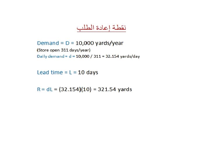
Reorder Point • Quantity to which inventory is allowed to drop before replenishment order is made • Need to order EOQ at the Reorder Point: ROP = d X LT d = Demand rate period LT = lead time in periods