Introduction to Spatial Computing Trends Spatiotemporal graphs Navigation

Introduction to Spatial Computing Trends: Spatio-temporal graphs

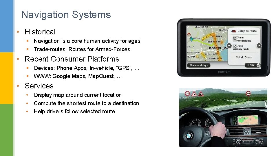
Navigation Systems • Historical § Navigation is a core human activity for ages! § Trade-routes, Routes for Armed-Forces • Recent Consumer Platforms § Devices: Phone Apps, In-vehicle, “GPS”, … § WWW: Google Maps, Map. Quest, … • Services • • • Display map around current location Compute the shortest route to a destination Help drivers follow selected route

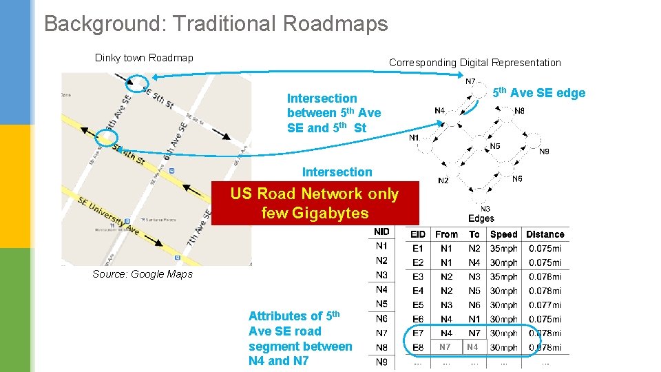
Background: Traditional Roadmaps Dinky town Roadmap Corresponding Digital Representation 5 th Ave SE edge Intersection between 5 th Ave SE and 5 th St Intersection between 5 th Ave Network only SE and 4 th St US Road few Gigabytes Source: Google Maps Attributes of 5 th Ave SE road segment between N 4 and N 7 N 4

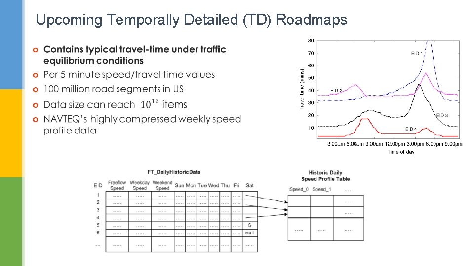
Upcoming Temporally Detailed (TD) Roadmaps Source: ESRI and NAVTEQ

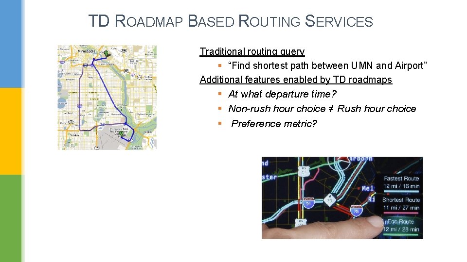
TD ROADMAP BASED ROUTING SERVICES Traditional routing query § “Find shortest path between UMN and Airport” Additional features enabled by TD roadmaps § At what departure time? § Non-rush hour choice ≠ Rush hour choice § Preference metric?

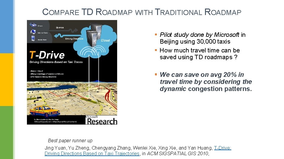
COMPARE TD ROADMAP WITH TRADITIONAL ROADMAP § Pilot study done by Microsoft in Beijing using 30, 000 taxis § How much travel time can be saved using TD roadmaps ? § We can save on avg 20% in travel time by considering the dynamic congestion patterns. Best paper runner up Jing Yuan, Yu Zheng, Chengyang Zhang, Wenlei Xie, Xing Xie, and Yan Huang, T-Drive: Driving Directions Based on Taxi Trajectories, in ACM SIGSPATIAL GIS 2010,

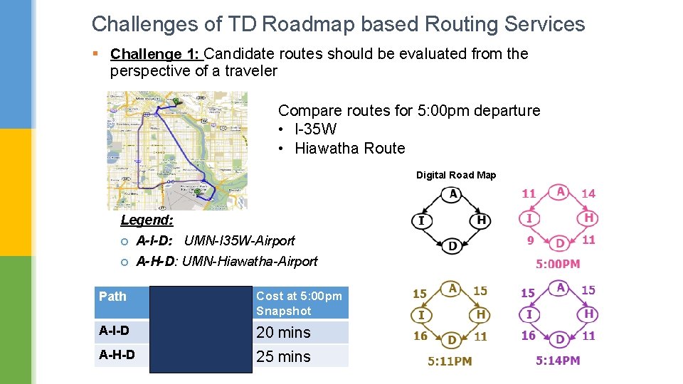
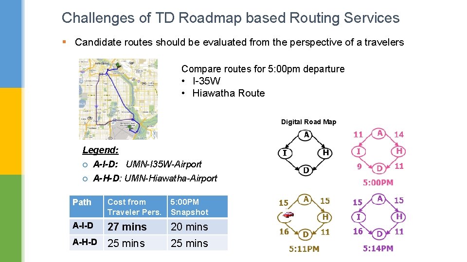
Challenges of TD Roadmap based Routing Services § Challenge 1: Candidate routes should be evaluated from the perspective of a traveler Compare routes for 5: 00 pm departure • I-35 W • Hiawatha Route Digital Road Map Legend: A-I-D: UMN-I 35 W-Airport A-H-D: UMN-Hiawatha-Airport Path Cost from Traveler Pers. Cost at 5: 00 pm Snapshot A-I-D 27 mins 20 mins A-H-D 25 mins

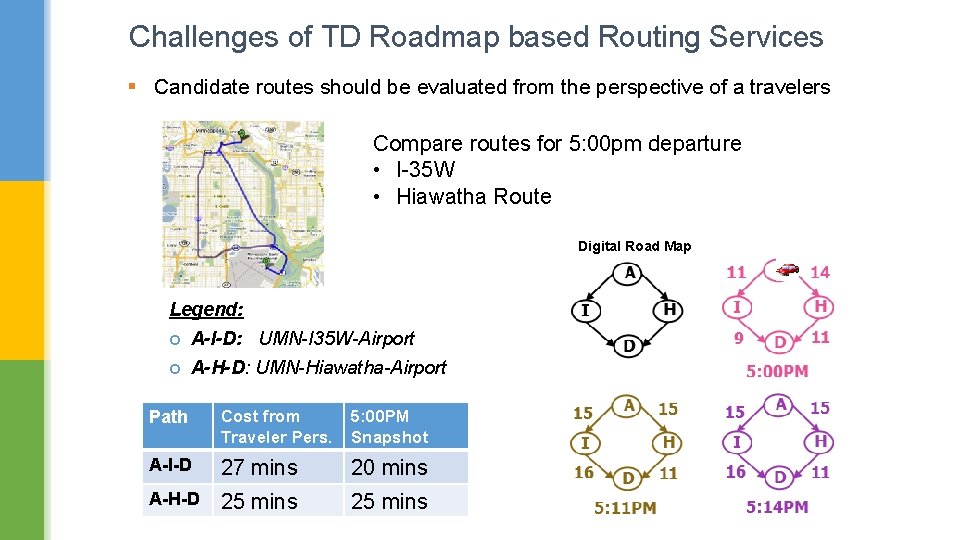
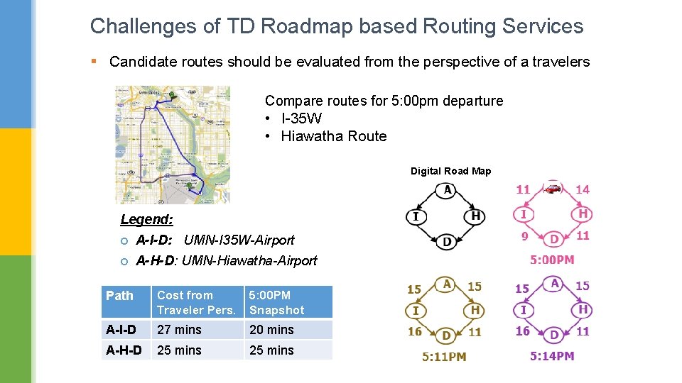
Challenges of TD Roadmap based Routing Services § Candidate routes should be evaluated from the perspective of a travelers Compare routes for 5: 00 pm departure • I-35 W • Hiawatha Route Digital Road Map Legend: A-I-D: UMN-I 35 W-Airport A-H-D: UMN-Hiawatha-Airport Path Cost from Traveler Pers. 5: 00 PM Snapshot A-I-D 27 mins 20 mins A-H-D 25 mins

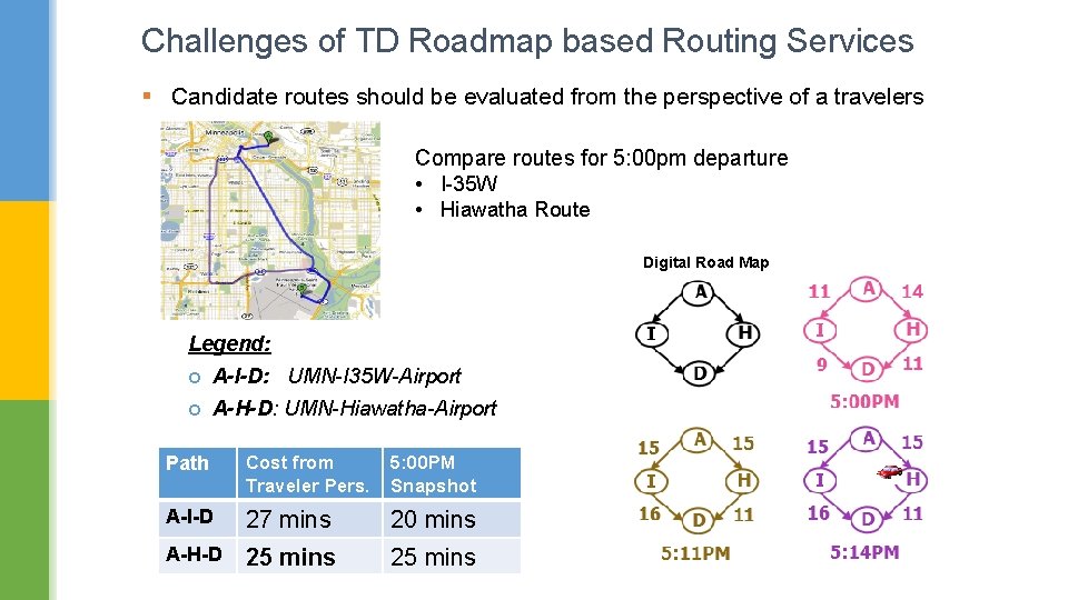
Challenges of TD Roadmap based Routing Services § Candidate routes should be evaluated from the perspective of a travelers Compare routes for 5: 00 pm departure • I-35 W • Hiawatha Route Digital Road Map Legend: A-I-D: UMN-I 35 W-Airport A-H-D: UMN-Hiawatha-Airport Path Cost from Traveler Pers. 5: 00 PM Snapshot A-I-D 27 mins 20 mins A-H-D 25 mins

Challenges of TD Roadmap based Routing Services § Candidate routes should be evaluated from the perspective of a travelers Compare routes for 5: 00 pm departure • I-35 W • Hiawatha Route Digital Road Map Legend: A-I-D: UMN-I 35 W-Airport A-H-D: UMN-Hiawatha-Airport Path Cost from Traveler Pers. 5: 00 PM Snapshot A-I-D 27 mins 20 mins A-H-D 25 mins

Challenges of TD Roadmap based Routing Services § Candidate routes should be evaluated from the perspective of a travelers Compare routes for 5: 00 pm departure • I-35 W • Hiawatha Route Digital Road Map Legend: A-I-D: UMN-I 35 W-Airport A-H-D: UMN-Hiawatha-Airport Path Cost from Traveler Pers. 5: 00 PM Snapshot A-I-D 27 mins 20 mins A-H-D 25 mins

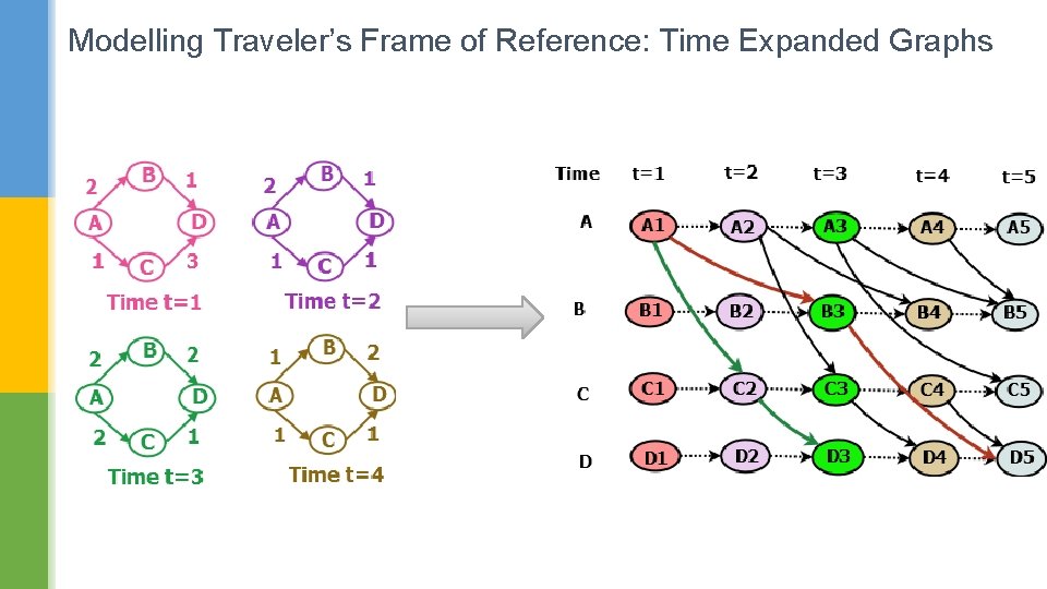
Modelling Traveler’s Frame of Reference: Time Expanded Graphs

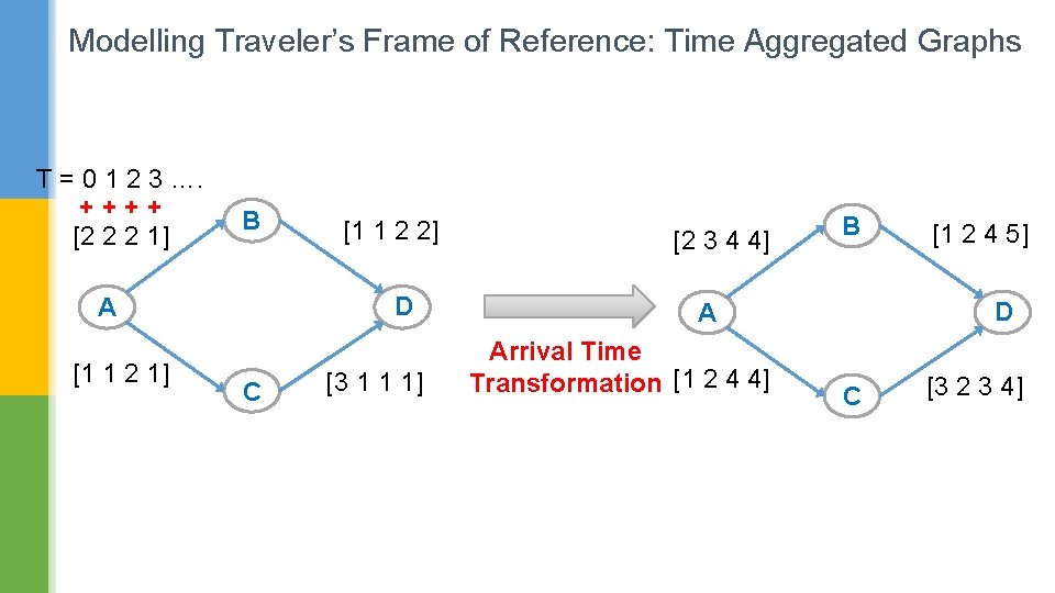
Modelling Traveler’s Frame of Reference: Time Aggregated Graphs [2 2 2 1] B D A [1 1 2 1] [1 1 2 2] C [3 1 1 1]

Modelling Traveler’s Frame of Reference: Time Aggregated Graphs T = 0 1 2 3 …. ++++ [2 2 2 1] B D A [1 1 2 1] [1 1 2 2] C [3 1 1 1] [2 3 4 4] B D A Arrival Time Transformation [1 2 4 4] [1 2 4 5] C [3 2 3 4]

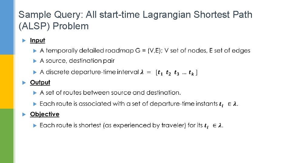
Sample Query: All start-time Lagrangian Shortest Path (ALSP) Problem

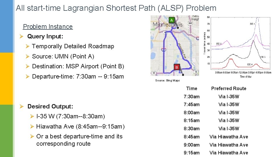
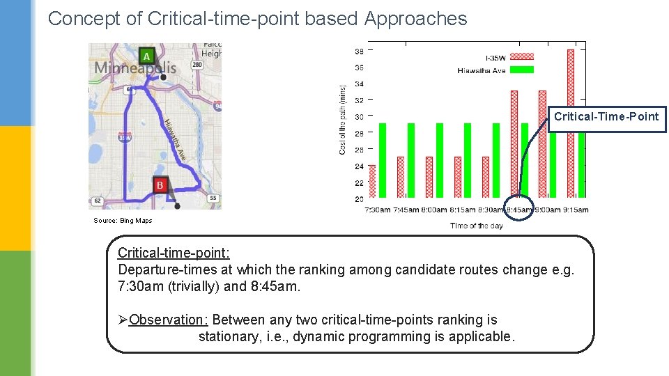
All start-time Lagrangian Shortest Path (ALSP) Problem Instance Ø Query Input: Ø Temporally Detailed Roadmap Ø Source: UMN (Point A) Ø Destination: MSP Airport (Point B) Ø Departure-time: 7: 30 am -- 9: 15 am Ø Desired Output: Ø I-35 W (7: 30 am--8: 30 am) Ø Hiawatha Ave (8: 45 am--9: 15 am) Ø Or a best departure-time and its corresponding route Source: Bing Maps Time Preferred Route 7: 30 am Via I-35 W 7: 45 am Via I-35 W 8: 00 am Via I-35 W 8: 15 am Via I-35 W 8: 30 am Via I-35 W 8: 45 am Via Hiawatha Ave 9: 00 am Via Hiawatha Ave 9: 15 am Via Hiawatha Ave

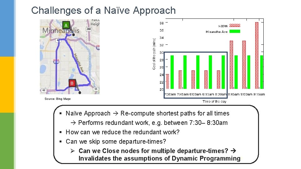
Challenges of a Naïve Approach Source: Bing Maps § Naïve Approach Re-compute shortest paths for all times Performs redundant work, e. g. between 7: 30– 8: 30 am § How can we reduce the redundant work? § Can we skip some departure-times? Ø Can we Close nodes for multiple departure-times? Invalidates the assumptions of Dynamic Programming!

Concept of Critical-time-point based Approaches Critical-Time-Point Source: Bing Maps Critical-time-point: Departure-times at which the ranking among candidate routes change e. g. 7: 30 am (trivially) and 8: 45 am. ØObservation: Between any two critical-time-points ranking is stationary, i. e. , dynamic programming is applicable.

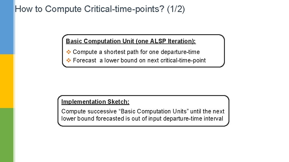
How to Compute Critical-time-points? (1/2) Basic Computation Unit (one ALSP Iteration): v Compute a shortest path for one departure-time v Forecast a lower bound on next critical-time-point Implementation Sketch: Compute successive “Basic Computation Units” until the next lower bound forecasted is out of input departure-time interval

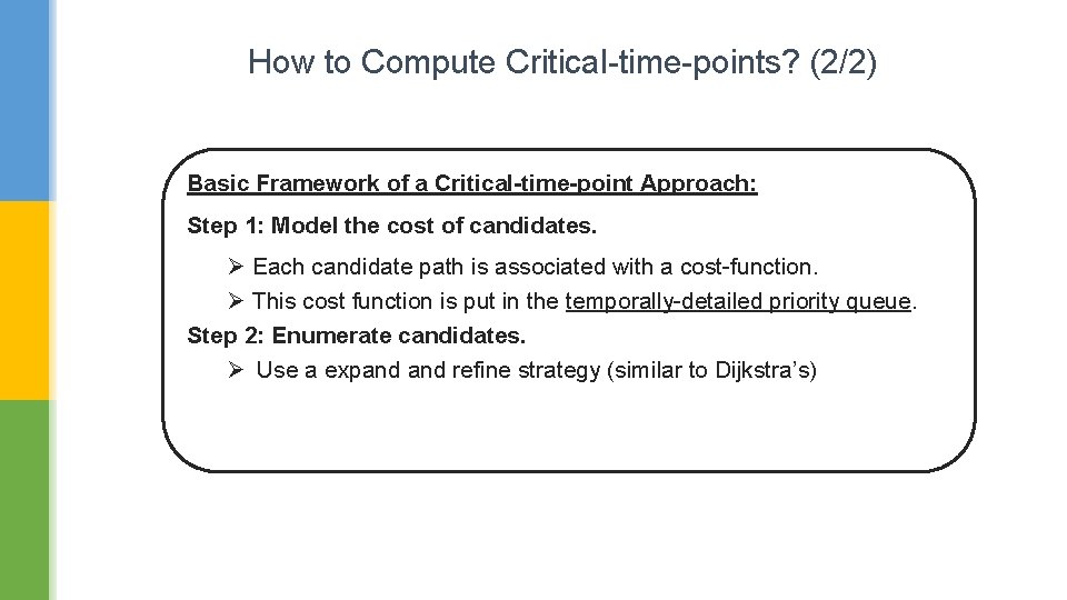
How to Compute Critical-time-points? (2/2) Basic Framework of a Critical-time-point Approach: Step 1: Model the cost of candidates. Ø Each candidate path is associated with a cost-function. Ø This cost function is put in the temporally-detailed priority queue. Step 2: Enumerate candidates. Ø Use a expand refine strategy (similar to Dijkstra’s)

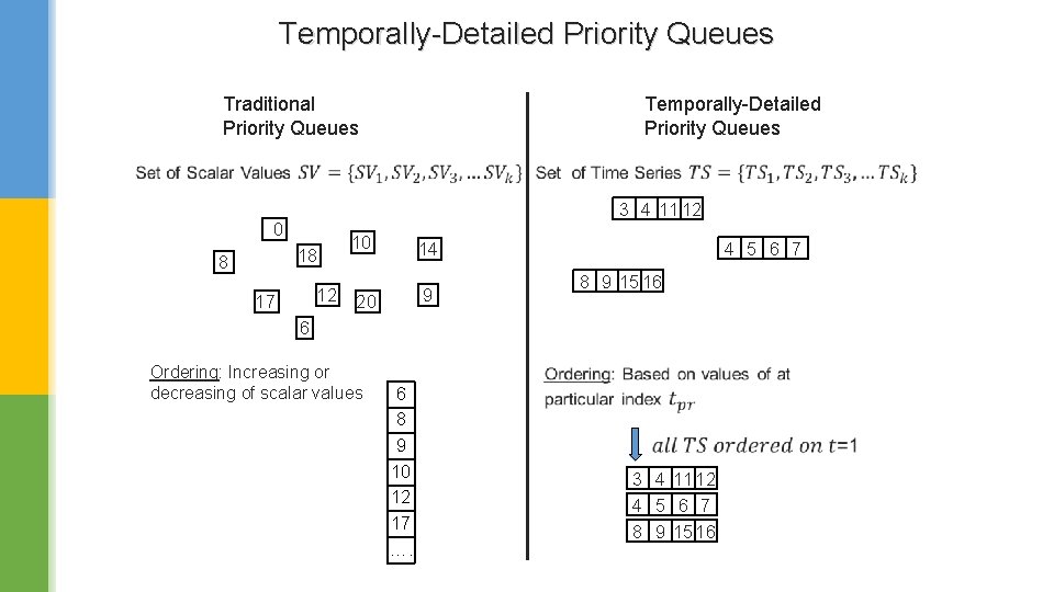
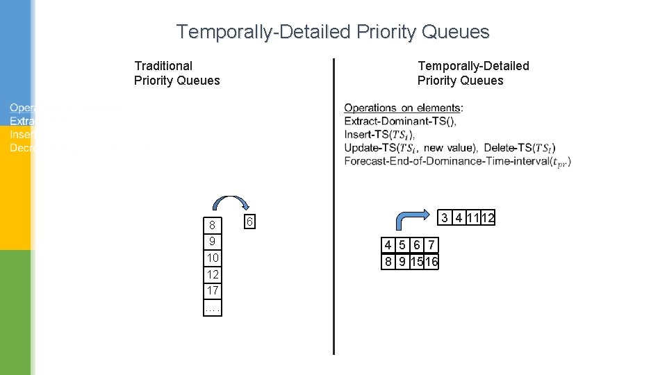
Temporally-Detailed Priority Queues Traditional Priority Queues 3 4 1112 30 18 8 Temporally-Detailed Priority Queues 12 17 10 14 20 9 4 5 6 7 8 9 1516 6 Ordering: Increasing or decreasing of scalar values 6 8 9 10 12 17 …. 3 4 1112 4 5 6 7 8 9 1516

Temporally-Detailed Priority Queues Traditional Priority Queues 8 9 10 12 17 …. 3 4 1112 6 4 5 6 7 8 9 1516

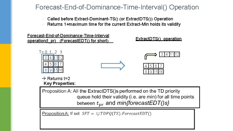
Forecast-End-of-Dominance-Time-Interval() Operation Ø Called before Extract-Dominant-TS() (or Extract. DTS()) Operation Ø Returns 1+maximum time for the current Extract-Min holds its validity Forecast-End-of-Dominance-Time-Interval operation(t_pr) (Forecast. EDT() for short) T= 0 1 2 3 3 4 1112 4 5 6 7 8 9 1516 Returns t=2 Key Properties: Extract. DTS() operation 3 4 1112 4 5 6 7 8 9 1516

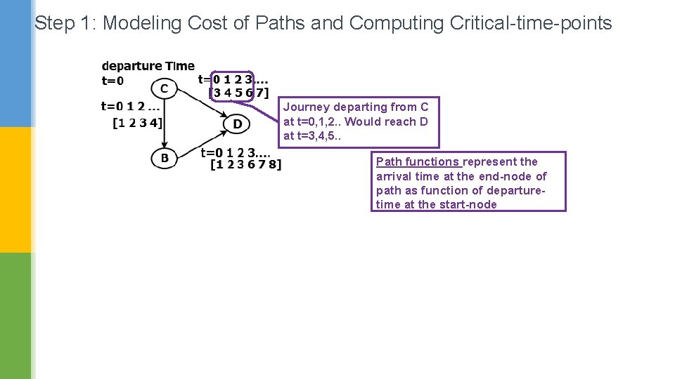
Step 1: Modeling Cost of Paths and Computing Critical-time-points Journey departing from C at t=0, 1, 2. . Would reach D at t=3, 4, 5. . Path functions represent the arrival time at the end-node of path as function of departuretime at the start-node

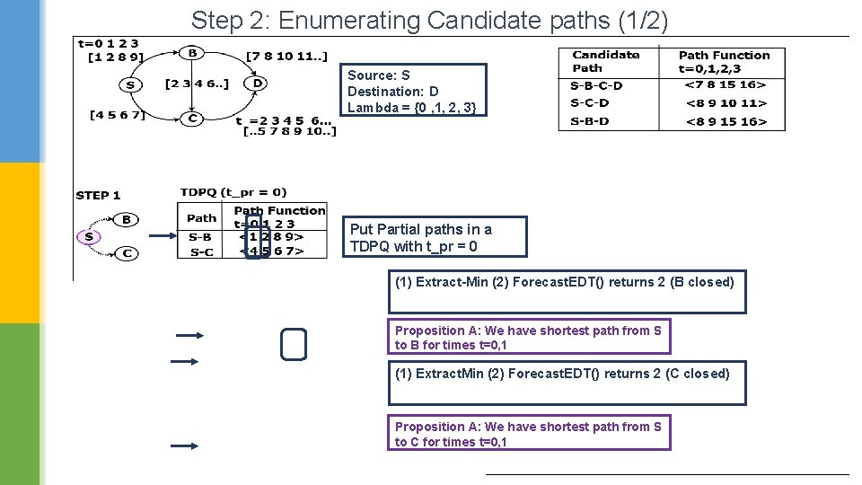
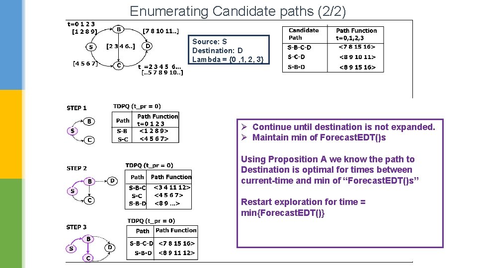
Step 2: Enumerating Candidate paths (1/2) Source: S Destination: D Lambda = {0 , 1, 2, 3} Put Partial paths in a TDPQ with t_pr = 0 (1) Extract-Min (2) Forecast. EDT() returns 2 (B closed) (3) Insert(S-B-C) and Insert(S-B-D) Proposition A: We have shortest path from S to B for times t=0, 1 (1) Extract. Min (2) Forecast. EDT() returns 2 (C closed) (3) Insert(S-B-C) and Insert(S-B-C-D) Proposition A: We have shortest path from S to C for times t=0, 1

Enumerating Candidate paths (2/2) Source: S Destination: D Lambda = {0 , 1, 2, 3} Ø Continue until destination is not expanded. Ø Maintain min of Forecast. EDT()s Using Proposition A we know the path to Destination is optimal for times between current-time and min of “Forecast. EDT()s” Restart exploration for time = min{Forecast. EDT()}

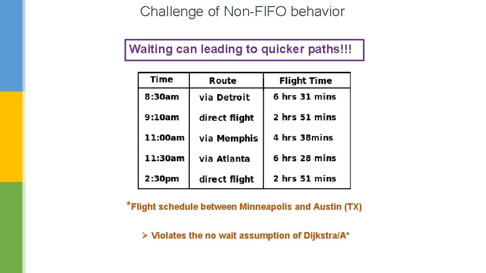
Challenge of Non-FIFO behavior Waiting can leading to quicker paths!!! *Flight schedule between Minneapolis and Austin (TX) Ø Violates the no wait assumption of Dijkstra/A*

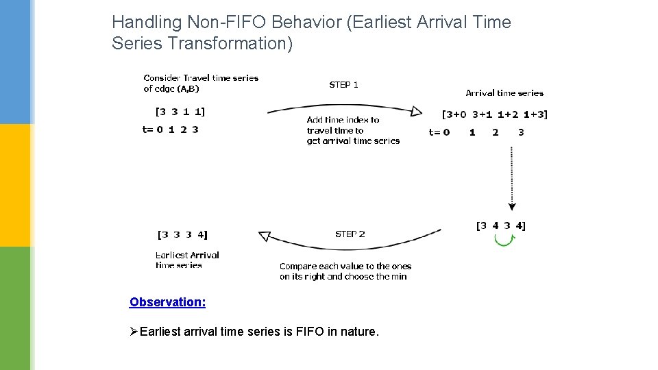
Handling Non-FIFO Behavior (Earliest Arrival Time Series Transformation) Observation: ØEarliest arrival time series is FIFO in nature.

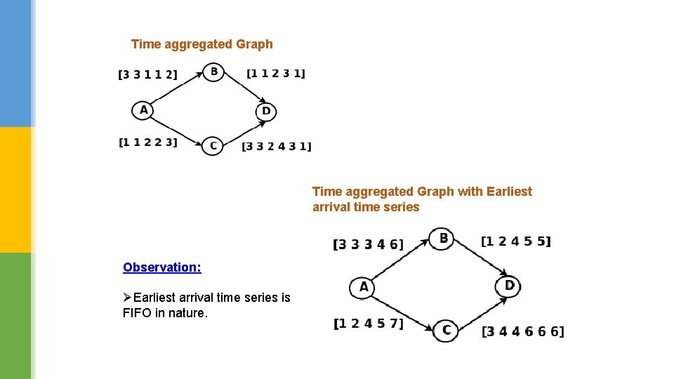
Time aggregated Graph with Earliest arrival time series Observation: ØEarliest arrival time series is FIFO in nature.