Planning and Navigation Competencies for Navigation Navigation is

Planning and Navigation

Competencies for Navigation • Navigation is composed of localization, mapping and motion planning Localization "Position" Global Map Environment Model Local Map Perception Cognition Path Real World Environment Motion Control – Different forms of motion planning inside the 6 cognition loop from R. Siegwart

Outline of this Lecture • Motion Planning – State-space and obstacle representation • Work space • Configuration space – Global motion planning • • Optimal control (not treated) Deterministic graph search Potential fields Probabilistic / random approaches – Local collision avoidance • • BUG VFH ND. . .

The Planning Problem (1/2) • The problem: find a path in the work space (physical space) from the initial position to the goal position avoiding all collisions with the obstacles • Assumption: there exists a good enough map of the environment for navigation. – Topological – Metric – Hybrid methods

The Planning Problem (2/2) • We can generally distinguish between – (global) path planning and – (local) obstacle avoidance. • First step: – Transformation of the map into a representation useful for planning – This step is planner-dependent • Second step: – Plan a path on the transformed map • Third step: – Send motion commands to controller – This step is planner-dependent (e. g. Model based feed forward, path following)

Map Representations Topological Map (Continuous Coordinates) Occupancy Grid Map (Discrete Coordinates) K-d Tree Map (Quadtree) Large memory requirement of grid maps - > k-d tree recursively breaks the environment into k pieces - Here k = 4, quadtree

Topological Map

Topological Maps +Edges can carry weights +Standard Graph Theory Algorithms (Dijkstra's algorithm) +Good abstract representation ●Several graphs for any world ●Assumption: Robot can travel between nodes ●Tradeoff in # of nodes: complexity vs. accuracy - Limited information

Grid World Two dimensional array of values Each cell represents a square of real world Typically a few centimeters to a few dozen centimeters

Alternative Representations Waste lots of bits for big open spaces KD-trees x<5 free y<5 occupied free

Quad. Tree Oct. Tree

Work Space Configuration Space Example: manipulator robots • State or configuration q can be described with k values qi • What is the configuration space of a mobile robot? Work Space Configuration Space: Planning in configuration space the dimension of this space is equal to the Degrees of Freedom (Do. F) of the robot

Configuration Space for a Mobile Robot • Mobile robots operating on a flat ground have 3 Do. F: (x, y, θ) • For simplification, in path planning mobile roboticists often assume that the robot is holonomic and that it is a point. In this way the configuration space is reduced to 2 D (x, y) • Because we have reduced each robot to a point, we have to inflate each obstacle by the size of the robot radius to compensate.

Configuration Space for a Mobile Robot

Path Planning: Overview of Algorithms 1. Optimal Control – Solves truly optimal solution – Becomes intractable for even moderately complex as well as nonconvex problems 2. Potential Field 3. Graph Search – Identify a set edges between nodes within the free space Source: http: //mitocw. udsm. ac. tz – Imposes a mathematical function over the state/configuration space – Many physical metaphors exist – Often employed due to its simplicity and similarity to optimal control solutions Configuration Space for a Mobile Robot – Where to put the nodes?

Potential Field Path Planning Strategies Khatib, 1986 • Robot is treated as a point under the influence of an artificial potential field. • Operates in the continuum – Generated robot movement is similar to a ball rolling down the hill – Goal generates attractive force – Obstacle are repulsive forces 6 - Planning and Navigation 6 16

Potential Fields Oussama Khatib, 1986. Model navigation as the sum of forces on the robot Goal: Attractive Force Large Distance --> Large Force Model as Spring Hooke's Law F = -k X Obstacles: Repulsive Force Small Distance --> Large Force Model as Electrically Charged Particles Coulomb's law F= k q 1 q 2 / r 2

attractive

repulsive

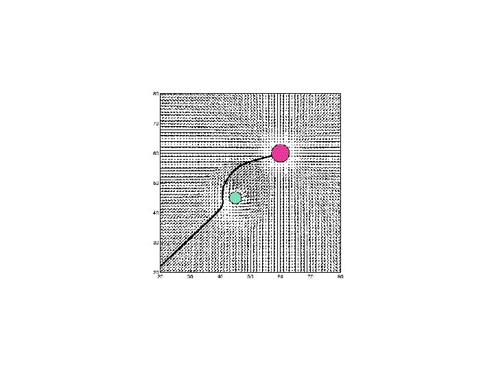
Potential Field Generation • Generation of potential field function U(q) • Generate artificial force field F(q) • Set robot speed (vx, vy) proportional to the force F(q) generated by the field – the force field drives the robot to the goal 6 - Planning and Navigation 6 21

Attractive Potential Field q = [x, y]T qgoal = [xgoal, ygoal]T • Parabolic function representing the Euclidean distance to the goal • Attracting force converges linearly towards 0 (goal) 6 - Planning and Navigation 6 22

Repulsing Potential Field • Should generate a barrier around all the obstacle – strong if close to the obstacle – not influence if far from the obstacle minimum distance to the object, ρ0 distance of influence of object Field is positive or zero and tends to infinity as q gets closer to the object obst. 6

Repulsive potential field

Potential Field Path Planning: • Notes: – Local minima problem exists – problem is getting more complex if the robot is not considered as a point mass – If objects are non-convex there exists situations where several minimal distances exist ® can result in oscillations 6 - Planning and Navigation 6 25

Computing the distance • In practice the distances are computed using sensors, such as range sensors which return the closets distance to obstacles

Graph Algorithms Methods – Breath First – Depth First – Dijkstra – A* and variants – D* and variants –. . .

Graph Construction: Cell Decomposition (1/4) • Divide space into simple, connected regions called cells • Determine which open cells are adjacent and construct a connectivity graph • Find cells in which the initial and goal configuration (state) lie and search for a path in the connectivity graph to join them. • From the sequence of cells found with an appropriate search algorithm, compute a path within each cell. – e. g. passing through the midpoints of cell boundaries or by sequence of wall following movements. • Possible cell decompositions: – Exact cell decomposition – Approximate cell decomposition: • • Fixed cell decomposition Adaptive cell decomposition 6 - Planning and Navigation

Graph Construction: Exact Cell Decomposition (2/4) 6 - Planning and Navigation 6 29

Graph Construction: Approximate Cell Decomposition (3/4) 6 - Planning and Navigation 6 30

Graph Construction: Adaptive Cell Decomposition (4/4) 6 - Planning and Navigation 6 31

Graph Search Strategies: Breadth-First Search 6

Dijkstra’s Algorithm A generic path planning problem from vertex I to vertex VI. The shortest path is I-II-III-V-VI with length 13. Often highly inefficient

Dijkstra’s Algorithm on a Grid

Graph Search Strategies: A* Search § Similar to Dijkstra‘s algorithm, except that it uses a heuristic function h(n) § f(n) = g(n) + ε h(n) 6 - Planning and Navigation 6 35

Dijkstra plus directional heuristic: A*

Graph Search Strategies: D* Search § Similar to A* search, except that th search starts from the goal outward § f(n) = g(n) + ε h(n) § First pass is identical to A* § Subsequent passes reuse information from previous searches § For example when after executing the algorithm for a few times, new obstacles appear.

Sampling-based Path Planning (or Randomized graph search) • When the state space is large complete solutions are often infeasible. • In practice, most algorithms are only resolution complete, i. e. , only complete if the resolution is ne-grained enough • Sampling-based planners create possible paths by randomly adding points to a tree until some solution is found

Rapidly Exploring Random Tree (RRT) § Well suited for high-dimensional search spaces § Often produces highly suboptimal solutions

Probabilistic Roadmaps (PRM) • create a tree by randomly sampling points in the state-space • test whether they are collision-free • connect them with neighboring points using paths that reflects the kinematics of a robot • use classical graph shortest path algorithms to find shortest paths on the resulting structure.

Planning at different length-scales

Take-home lessons • First step in addressing a planning problem is choosing a suitable map representation • Reduce robot to a point-mass by inflating obstacles • Grid-based algorithms are complete, sampling-based ones probabilistically complete, but usually faster • Most real planning problems require combination of multiple algorithms

Obstacle Avoidance (Local Path Planning) • tacle n obs p) s (ma rved o b se l e ac o b st w(t) ath ed p Plan – the overall goal – the actual speed and kinematics of the robot – the on boards sensors – the actual and future risk of collision v(t), • know • • The goal of the obstacle avoidance algorithms is to avoid collisions with obstacles It is usually based on a local map Often implemented as a more or less independent task However, efficient obstacle avoidance should be optimal with respect to • Example: Alice 6 - Planning and Navigation 6 43

Obstacle Avoidance: Bug 1 • Following along the obstacle to avoid it • Each encountered obstacle is once fully circled before it is left at the point closest to the goal • Advantages – No global map required – Completeness guaranteed • Disadvantages – Solutions are often highly suboptimal 6 - Planning and Navigation 6 44

Obstacle Avoidance: Bug 2 • Following the obstacle always on the left or right side • Leaving the obstacle if the direct connection between start and goal is crossed 6 - Planning and Navigation 6 45